Predict housing prices 🏠 in Austin TX with xgboost

This is the latest in my series of screencasts demonstrating how to use the tidymodels packages, from just getting started to tuning more complex models. My screencasts lately have focused on xgboost as I have participated in SLICED, a competitive data science streaming show. This past week were the semifinals, where we competed to predict prices of homes in Austin, TX. 🏠 One of the more interesting available variables for this dataset was the text description of the real estate listings, so let’s walk through one way to incorporate text information with boosted tree modeling.

Here is the code I used in the video, for those who prefer reading instead of or in addition to video.

Explore data

Our modeling goal is to predict the price (binned) for homes in Austin, TX given features about the real estate listing. This is a multiclass classification challenge, where we needed to submit a probability for each home being in each priceRange bin. The main data set provided is in a CSV file called training.csv.

library(tidyverse)
train_raw <- read_csv("train.csv")

train_raw %>%
  count(priceRange)


## # A tibble: 5 × 2
## priceRange n
## <chr> <int>
## 1 0-250000 1249
## 2 250000-350000 2356
## 3 350000-450000 2301
## 4 450000-650000 2275
## 5 650000+ 1819

You can watch this week’s full episode of SLICED to see lots of exploratory data analysis and visualization of this dataset, but let’s just make a few data visualization for context in this blog post.

How is price distributed across Austin?

price_plot <-
  train_raw %>%
  mutate(priceRange = parse_number(priceRange)) %>%
  ggplot(aes(longitude, latitude, z = priceRange)) +
  stat_summary_hex(alpha = 0.8, bins = 50) +
  scale_fill_viridis_c() +
  labs(
    fill = "mean",
    title = "Price"
  )

price_plot

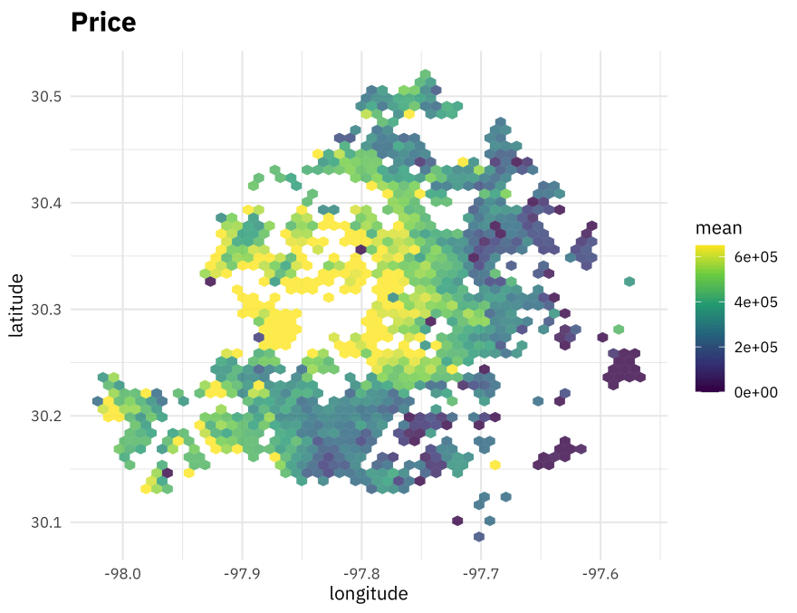
Let’s look at this distribution and compare it to some other variables available in the dataset. We can create a little plotting function using {{}} to quickly iterate through, and put them together with patchwork.

library(patchwork)

plot_austin <- function(var, title) {
  train_raw %>%
    ggplot(aes(longitude, latitude, z = {{ var }})) +
    stat_summary_hex(alpha = 0.8, bins = 50) +
    scale_fill_viridis_c() +
    labs(
      fill = "mean",
      title = title
    )
}

(price_plot + plot_austin(avgSchoolRating, "School rating")) /
  (plot_austin(yearBuilt, "Year built") + plot_austin(log(lotSizeSqFt), "Lot size (log)"))

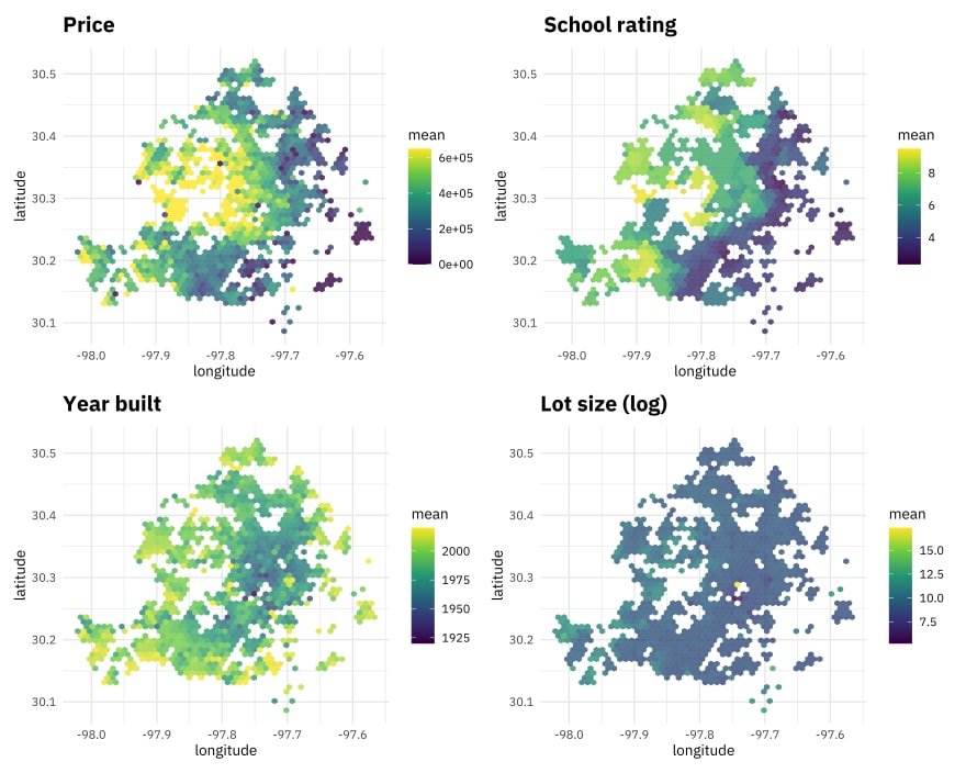
Notice the east/west gradients as well as the radial changes. I went to grad school in Austin and this all look very familiar to me!

Finding words related to price

The description variable contains text from each real estate listing. We could try to use the text features directly in modeling, as described in our book, but I’ve found that often isn’t great for boosted tree models (which tend to be what works best overall in an environment like SLICED). Let’s walk through another option which may work better in some situations, which is to use some separate analysis to identify important words and then create dummy variables indicating whether any given listing has those words.

Let’s start by tidying the description text.

library(tidytext)

austin_tidy <-
  train_raw %>%
  mutate(priceRange = parse_number(priceRange) + 100000) %>%
  unnest_tokens(word, description) %>%
  anti_join(get_stopwords())

austin_tidy %>%
  count(word, sort = TRUE)


## # A tibble: 17,944 × 2
## word n
## <chr> <int>
## 1 home 11620
## 2 kitchen 5721
## 3 room 5494
## 4 austin 4918
## 5 new 4772
## 6 large 4771
## 7 2 4585
## 8 bedrooms 4571
## 9 contains 4413
## 10 3 4386
## # … with 17,934 more rows

Next, let’s compute word frequencies per price range for the top 100 words.

top_words <-
  austin_tidy %>%
  count(word, sort = TRUE) %>%
  filter(!word %in% as.character(1:5)) %>%
  slice_max(n, n = 100) %>%
  pull(word)

word_freqs <-
  austin_tidy %>%
  count(word, priceRange) %>%
  complete(word, priceRange, fill = list(n = 0)) %>%
  group_by(priceRange) %>%
  mutate(
    price_total = sum(n),
    proportion = n / price_total
  ) %>%
  ungroup() %>%
  filter(word %in% top_words)

word_freqs


## # A tibble: 500 × 5
## word priceRange n price_total proportion
## <chr> <dbl> <dbl> <dbl> <dbl>
## 1 access 100000 180 56290 0.00320
## 2 access 350000 365 114853 0.00318
## 3 access 450000 322 116678 0.00276
## 4 access 550000 294 125585 0.00234
## 5 access 750000 248 112073 0.00221
## 6 appliances 100000 209 56290 0.00371
## 7 appliances 350000 583 114853 0.00508
## 8 appliances 450000 576 116678 0.00494
## 9 appliances 550000 567 125585 0.00451
## 10 appliances 750000 391 112073 0.00349
## # … with 490 more rows

Now let’s use modeling to find the words that are increasing with price and those that are decreasing with price.

word_mods <-
  word_freqs %>%
  nest(data = c(priceRange, n, price_total, proportion)) %>%
  mutate(
    model = map(data, ~ glm(cbind(n, price_total) ~ priceRange, ., family = "binomial")),
    model = map(model, tidy)
  ) %>%
  unnest(model) %>%
  filter(term == "priceRange") %>%
  mutate(p.value = p.adjust(p.value)) %>%
  arrange(-estimate)

word_mods


## # A tibble: 100 × 7
## word data term estimate std.error statistic p.value
## <chr> <list> <chr> <dbl> <dbl> <dbl> <dbl>
## 1 outdoor <tibble [5 × 4]> priceRange 0.00000325 1.85e-7 17.6 4.37e-67
## 2 custom <tibble [5 × 4]> priceRange 0.00000214 1.47e-7 14.6 3.98e-46
## 3 pool <tibble [5 × 4]> priceRange 0.00000159 1.22e-7 13.0 6.12e-37
## 4 office <tibble [5 × 4]> priceRange 0.00000150 1.46e-7 10.3 6.03e-23
## 5 suite <tibble [5 × 4]> priceRange 0.00000143 1.39e-7 10.3 4.03e-23
## 6 gorgeous <tibble [5 × 4]> priceRange 0.000000975 1.62e-7 6.02 1.19e- 7
## 7 w <tibble [5 × 4]> priceRange 0.000000920 9.05e-8 10.2 2.33e-22
## 8 windows <tibble [5 × 4]> priceRange 0.000000890 1.28e-7 6.95 2.81e-10
## 9 private <tibble [5 × 4]> priceRange 0.000000889 1.15e-7 7.70 1.08e-12
## 10 car <tibble [5 × 4]> priceRange 0.000000778 1.66e-7 4.69 1.52e- 4
## # … with 90 more rows

Let’s make something like a volcano plot to see the relationship between p-value and effect size for these words.

library(ggrepel)

word_mods %>%
  ggplot(aes(estimate, p.value)) +
  geom_vline(xintercept = 0, lty = 2, alpha = 0.7, color = "gray50") +
  geom_point(color = "midnightblue", alpha = 0.8, size = 2.5) +
  scale_y_log10() +
  geom_text_repel(aes(label = word), family = "IBMPlexSans")

• Words like outdoor, custom, pool, suite, office increase with price.
• Words like new, paint, carpet, great, tile, close, flooring decrease with price.

These are the words that we’d like to try to detect and use in feature engineering for our xgboost model, rather than using all the text tokens as features individually.

higher_words <-
  word_mods %>%
  filter(p.value < 0.05) %>%
  slice_max(estimate, n = 12) %>%
  pull(word)

lower_words <-
  word_mods %>%
  filter(p.value < 0.05) %>%
  slice_max(-estimate, n = 12) %>%
  pull(word)

We can look at these changes with price directly. For example, these are the words most associated with price decrease.

word_freqs %>%
  filter(word %in% lower_words) %>%
  ggplot(aes(priceRange, proportion, color = word)) +
  geom_line(size = 2.5, alpha = 0.7, show.legend = FALSE) +
  facet_wrap(vars(word), scales = "free_y") +
  scale_x_continuous(labels = scales::dollar) +
  scale_y_continuous(labels = scales::percent, limits = c(0, NA)) +
  labs(x = NULL, y = "proportion of total words used for homes at that price") +
  theme_light(base_family = "IBMPlexSans")

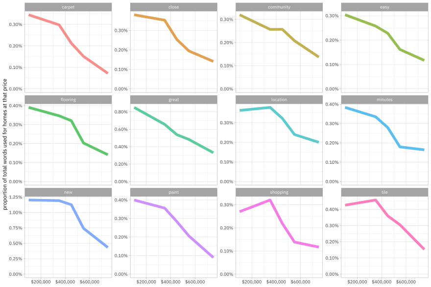
Cheaper houses are “great” but not expensive houses, and apparently you don’t need to mention the location (“close,” “minutes,” “location”) of more expensive houses.

Build a model

Let’s start our modeling by setting up our “data budget,” as well as the metrics (this challenge was evaluate on multiclass log loss).

library(tidymodels)

set.seed(123)
austin_split <- train_raw %>%
  select(-city) %>%
  mutate(description = str_to_lower(description)) %>%
  initial_split(strata = priceRange)
austin_train <- training(austin_split)
austin_test <- testing(austin_split)
austin_metrics <- metric_set(accuracy, roc_auc, mn_log_loss)

set.seed(234)
austin_folds <- vfold_cv(austin_train, v = 5, strata = priceRange)
austin_folds


## # 5-fold cross-validation using stratification 
## # A tibble: 5 × 2
## splits id   
## <list> <chr>
## 1 <split [5996/1502]> Fold1
## 2 <split [5998/1500]> Fold2
## 3 <split [5999/1499]> Fold3
## 4 <split [5999/1499]> Fold4
## 5 <split [6000/1498]> Fold5

For feature engineering, let’s use basically everything in the dataset (aside from city, which was not a very useful variable) and create dummy or indicator variables using step_regex(). The idea here is that we will detect whether these words associated with low/high price are there and create a yes/no variable indicating their presence or absence.

higher_pat <- glue::glue_collapse(higher_words, sep = "|")
lower_pat <- glue::glue_collapse(lower_words, sep = "|")

austin_rec <-
  recipe(priceRange ~ ., data = austin_train) %>%
  update_role(uid, new_role = "uid") %>%
  step_regex(description, pattern = higher_pat, result = "high_price_words") %>%
  step_regex(description, pattern = lower_pat, result = "low_price_words") %>%
  step_rm(description) %>%
  step_novel(homeType) %>%
  step_unknown(homeType) %>%
  step_other(homeType, threshold = 0.02) %>%
  step_dummy(all_nominal_predictors()) %>%
  step_nzv(all_predictors())

austin_rec


## Data Recipe
## 
## Inputs:
## 
## role #variables
## outcome 1
## predictor 13
## uid 1
## 
## Operations:
## 
## Regular expression dummy variable using `outdoor|custom|pool|office|suite|gorgeous|w|windows|private|car|high|full`
## Regular expression dummy variable using `carpet|paint|close|flooring|shopping|new|easy|minutes|tile|great|community|location`
## Delete terms description
## Novel factor level assignment for homeType
## Unknown factor level assignment for homeType
## Collapsing factor levels for homeType
## Dummy variables from all_nominal_predictors()
## Sparse, unbalanced variable filter on all_predictors()

Now let’s create a tunable xgboost model specification, tuning a lot of the important model hyperparameters, and combine it with our feature engineering recipe in a workflow(). We can also create a custom xgb_grid to specify what parameters I want to try out, like not-too-small learning rate, avoiding tree stubs, etc. I chose this parameter grid to get reasonable performance in a reasonable amount of tuning time.

xgb_spec <-
  boost_tree(
    trees = 1000,
    tree_depth = tune(),
    min_n = tune(),
    mtry = tune(),
    sample_size = tune(),
    learn_rate = tune()
  ) %>%
  set_engine("xgboost") %>%
  set_mode("classification")

xgb_word_wf <- workflow(austin_rec, xgb_spec)

set.seed(123)
xgb_grid <-
  grid_max_entropy(
    tree_depth(c(5L, 10L)),
    min_n(c(10L, 40L)),
    mtry(c(5L, 10L)),
    sample_prop(c(0.5, 1.0)),
    learn_rate(c(-2, -1)),
    size = 20
  )

xgb_grid


## # A tibble: 20 × 5
## tree_depth min_n mtry sample_size learn_rate
## <int> <int> <int> <dbl> <dbl>
## 1 7 33 8 0.768 0.0845
## 2 10 33 7 0.928 0.0784
## 3 5 21 6 0.626 0.0868
## 4 9 31 8 0.728 0.0162
## 5 8 35 5 0.666 0.0937
## 6 6 21 5 0.907 0.0105
## 7 6 27 6 0.982 0.0729
## 8 7 33 8 0.936 0.0102
## 9 7 15 5 0.559 0.0182
## 10 6 35 9 0.784 0.0347
## 11 9 39 9 0.737 0.0582
## 12 8 17 8 0.596 0.0818
## 13 9 21 7 0.601 0.0136
## 14 7 15 7 0.763 0.0197
## 15 6 12 10 0.800 0.0569
## 16 9 19 9 0.589 0.0138
## 17 10 14 5 0.829 0.0140
## 18 8 37 10 0.664 0.0202
## 19 5 11 5 0.514 0.0136
## 20 10 38 9 0.962 0.0150

Now we can tune across the grid of parameters and our resamples. Since we are trying quite a lot of hyperparameter combinations, let’s use racing to quit early on clearly bad hyperparameter combinations.

library(finetune)
doParallel::registerDoParallel()

set.seed(234)
xgb_word_rs <-
  tune_race_anova(
    xgb_word_wf,
    austin_folds,
    grid = xgb_grid,
    metrics = metric_set(mn_log_loss),
    control = control_race(verbose_elim = TRUE)
  )

xgb_word_rs


## # Tuning results
## # 5-fold cross-validation using stratification 
## # A tibble: 5 × 5
## splits id .order .metrics .notes          
## <list> <chr> <int> <list> <list>          
## 1 <split [5996/1502]> Fold1 3 <tibble [20 × 9]> <tibble [0 × 1]>
## 2 <split [5999/1499]> Fold3 1 <tibble [20 × 9]> <tibble [0 × 1]>
## 3 <split [6000/1498]> Fold5 2 <tibble [20 × 9]> <tibble [0 × 1]>
## 4 <split [5999/1499]> Fold4 4 <tibble [10 × 9]> <tibble [0 × 1]>
## 5 <split [5998/1500]> Fold2 5 <tibble [4 × 9]> <tibble [0 × 1]>

That takes a little while but we did it!

Evaluate results

First off, how did the “race” go?

plot_race(xgb_word_rs)

We can look at the top results manually as well.

show_best(xgb_word_rs)


## # A tibble: 4 × 11
## mtry min_n tree_depth learn_rate sample_size .metric .estimator mean n
## <int> <int> <int> <dbl> <dbl> <chr> <chr> <dbl> <int>
## 1 5 14 10 0.0140 0.829 mn_log_l… multiclass 0.920 5
## 2 7 15 7 0.0197 0.763 mn_log_l… multiclass 0.921 5
## 3 5 15 7 0.0182 0.559 mn_log_l… multiclass 0.921 5
## 4 9 19 9 0.0138 0.589 mn_log_l… multiclass 0.923 5
## # … with 2 more variables: std_err <dbl>, .config <chr>

Let’s use last_fit() to fit one final time to the training data and evaluate one final time on the testing data, with the numerically optimal result from xgb_word_rs.

xgb_last <-
  xgb_word_wf %>%
  finalize_workflow(select_best(xgb_word_rs, "mn_log_loss")) %>%
  last_fit(austin_split)

xgb_last


## # Resampling results
## # Manual resampling 
## # A tibble: 1 × 6
## splits id .metrics .notes .predictions .workflow
## <list> <chr> <list> <list> <list> <list>   
## 1 <split [7498/2502]> train/test split <tibble … <tibble… <tibble [2,… <workflo…

How did this model perform on the testing data, that was not used in tuning/training?

collect_predictions(xgb_last) %>%
  mn_log_loss(priceRange, `.pred_0-250000`:`.pred_650000+`)


## # A tibble: 1 × 3
## .metric .estimator .estimate
## <chr> <chr> <dbl>
## 1 mn_log_loss multiclass 0.910

This result is pretty good for a single (not ensembled) model and is a wee bit better than what I did during the SLICED competition. I had an R bomb right as I was finishing up tuning a model just like the one I am demonstrating here!

How does this model perform across the different classes?

collect_predictions(xgb_last) %>%
  conf_mat(priceRange, .pred_class) %>%
  autoplot()

We can also visualize this with an ROC curve.

collect_predictions(xgb_last) %>%
  roc_curve(priceRange, `.pred_0-250000`:`.pred_650000+`) %>%
  ggplot(aes(1 - specificity, sensitivity, color = .level)) +
  geom_abline(lty = 2, color = "gray80", size = 1.5) +
  geom_path(alpha = 0.8, size = 1.2) +
  coord_equal() +
  labs(color = NULL)

Notice that it is easier to identify the most expensive homes but more difficult to correctly classify the less expensive homes.

What features are most important for this xgboost model?

library(vip)
extract_workflow(xgb_last) %>%
  extract_fit_parsnip() %>%
  vip(geom = "point", num_features = 15)

The spatial information in latitude/longitude are by far the most important. Notice that the model uses low_price_words more than it uses, for example, whether there is a spa or whether it is a single family home (as opposed to a townhome or condo). It looks like the model is trying to distinguish some of those lower priced categories. The model does not really use the high_price_words variable, perhaps because it is already easy to find the expensive houses.

The two finalists from SLICED go on to compete next Tuesday, which should be fun and interesting to watch! I have enjoyed the opportunity to participate this season.