
Lately I’ve been publishing screencasts demonstrating how to use the tidymodels framework, from first steps in modeling to how to evaluate complex models. Today’s screencast focuses on using bootstrap resampling with this week’s #TidyTuesday dataset from the Claremont Run Project about issues of the comic book series Uncanny X-Men. 🦸
Here is the code I used in the video, for those who prefer reading instead of or in addition to video.
Read in the data
Our modeling goal is to use information about speech bubbles, thought bubbles, narrative statements, and character depictions from this week’s #TidyTuesday dataset to understand more about characteristics of individual comic book issues. Let’s focus on two modeling questions.
- Does a given issue have the X-Mansion as a location?
- Does a given issue pass the Bechdel test?
We’re going to use three of the datasets from this week.
library(tidyverse)

character_visualization <- readr::read_csv("https://raw.githubusercontent.com/rfordatascience/tidytuesday/master/data/2020/2020-06-30/character_visualization.csv")
xmen_bechdel <- readr::read_csv("https://raw.githubusercontent.com/rfordatascience/tidytuesday/master/data/2020/2020-06-30/xmen_bechdel.csv")
locations <- readr::read_csv("https://raw.githubusercontent.com/rfordatascience/tidytuesday/master/data/2020/2020-06-30/locations.csv")
The character_visualization dataset counts up each time one of the main 25 character speaks, thinks, is involved in narrative statements, or is depicted total.
character_visualization


## # A tibble: 9,800 x 7
## issue costume character speech thought narrative depicted
## <dbl> <chr> <chr> <dbl> <dbl> <dbl> <dbl>
## 1 97 Costume Editor narration 0 0 0 0
## 2 97 Costume Omnipresent narration 0 0 0 0
## 3 97 Costume Professor X = Charles Xavier… 0 0 0 0
## 4 97 Costume Wolverine = Logan 7 0 0 10
## 5 97 Costume Cyclops = Scott Summers 24 3 0 23
## 6 97 Costume Marvel Girl/Phoenix = Jean G… 0 0 0 0
## 7 97 Costume Storm = Ororo Munroe 11 0 0 9
## 8 97 Costume Colossus = Peter (Piotr) Ras… 9 0 0 17
## 9 97 Costume Nightcrawler = Kurt Wagner 10 0 0 17
## 10 97 Costume Banshee = Sean Cassidy 0 0 0 5
## # … with 9,790 more rows
Let’s aggregate this dataset to the issue level so we can build models using per-issue differences in speaking, thinking, narrative, and total depictions.
per_issue <- character_visualization %>%
  group_by(issue) %>%
  summarise(across(speech:depicted, sum)) %>%
  ungroup()

per_issue


## # A tibble: 196 x 5
## issue speech thought narrative depicted
## <dbl> <dbl> <dbl> <dbl> <dbl>
## 1 97 146 13 71 168
## 2 98 172 9 29 180
## 3 99 105 22 29 124
## 4 100 141 28 7 122
## 5 101 158 27 58 191
## 6 102 78 27 33 133
## 7 103 91 6 25 121
## 8 104 142 15 25 165
## 9 105 83 12 24 128
## 10 106 20 6 20 16
## # … with 186 more rows
I’m not doing a ton of EDA here but there are lots of great examples out there to explore on Twitter!
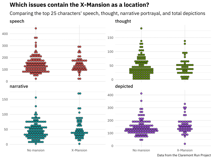
Which issues have the X-Mansion as a location?
Let’s start with our first model. The X-Mansion is the most frequently used location, but it does not appear in every episode.
x_mansion <- locations %>%
  group_by(issue) %>%
  summarise(mansion = "X-Mansion" %in% location)

locations_joined <- per_issue %>%
  inner_join(x_mansion)

locations_joined %>%
  mutate(mansion = if_else(mansion, "X-Mansion", "No mansion")) %>%
  pivot_longer(speech:depicted, names_to = "visualization") %>%
  mutate(visualization = fct_inorder(visualization)) %>%
  ggplot(aes(mansion, value, fill = visualization)) +
  geom_dotplot(
    binaxis = "y", stackdir = "center",
    binpositions = "all",
    show.legend = FALSE
  ) +
  facet_wrap(~visualization, scales = "free_y") +
  labs(
    x = NULL, y = NULL,
    title = "Which issues contain the X-Mansion as a location?",
    subtitle = "Comparing the top 25 characters' speech, thought, narrative portrayal, and total depictions",
    caption = "Data from the Claremont Run Project"
  )
Now let’s create bootstrap resamples and fit a logistic regression model to each resample. What are the bootstrap confidence intervals on the model parameters?
library(tidymodels)
set.seed(123)
boots <- bootstraps(locations_joined, times = 1000, apparent = TRUE)

boot_models <- boots %>%
  mutate(
    model = map(
      splits,
      ~ glm(mansion ~ speech + thought + narrative + depicted,
        family = "binomial", data = analysis(.)
      )
    ),
    coef_info = map(model, tidy)
  )

boot_coefs <- boot_models %>%
  unnest(coef_info)

int_pctl(boot_models, coef_info)


## # A tibble: 5 x 6
## term .lower .estimate .upper .alpha .method
## <chr> <dbl> <dbl> <dbl> <dbl> <chr>
## 1 (Intercept) -2.42 -1.29 -0.277 0.05 percentile
## 2 depicted 0.00193 0.0103 0.0196 0.05 percentile
## 3 narrative -0.0106 0.00222 0.0143 0.05 percentile
## 4 speech -0.0148 -0.00716 0.000617 0.05 percentile
## 5 thought -0.0143 -0.00338 0.00645 0.05 percentile
How are the parameters distributed?
boot_coefs %>%
  filter(term != "(Intercept)") %>%
  mutate(term = fct_inorder(term)) %>%
  ggplot(aes(estimate, fill = term)) +
  geom_vline(
    xintercept = 0, color = "gray50",
    alpha = 0.6, lty = 2, size = 1.5
  ) +
  geom_histogram(alpha = 0.8, bins = 25, show.legend = FALSE) +
  facet_wrap(~term, scales = "free") +
  labs(
    title = "Which issues contain the X-Mansion as a location?",
    subtitle = "Comparing the top 25 characters' speech, thought, narrative portrayal, and total depictions",
    caption = "Data from the Claremont Run Project"
  )

- Issues with more depictions of the main 25 characters (i.e. large groups of X-Men) are more likely to occur in the X-Mansion.
- Issues with more speech bubbles from these characters are less likely to occur in the X-Mansion.
Apparently issues with lots of talking are more likely to occur elsewhere!
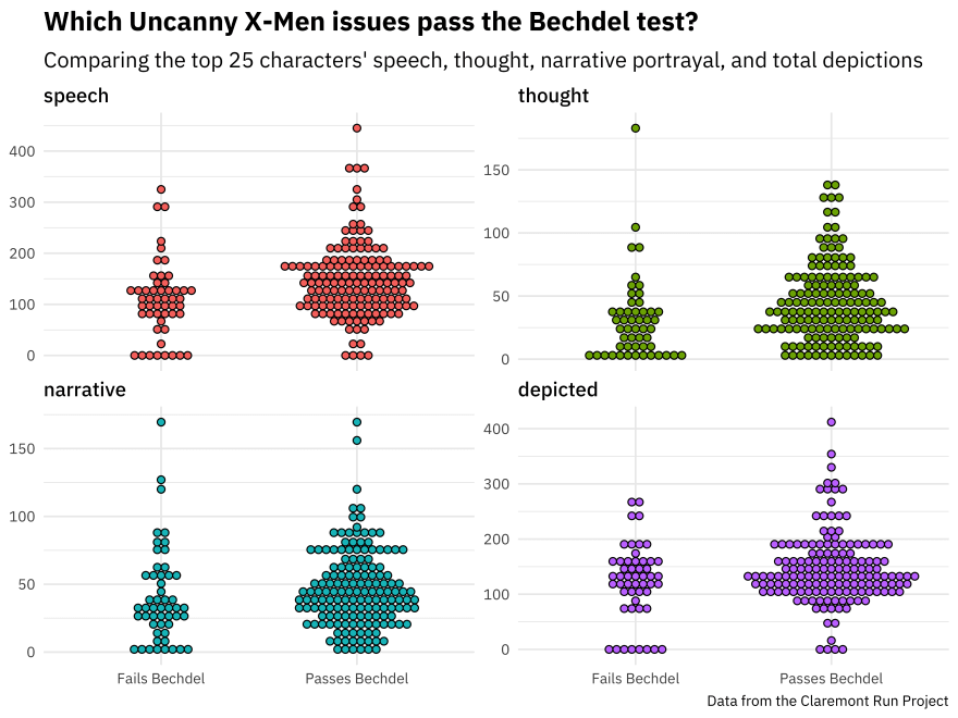
Now let’s do the Bechdel test
If you haven’t heard about the Bechdel test, this video (now over 10 years old!) is a nice explainer. We can use the same approach from the previous section but replace the data about issue locations with the Bechdel test data.
bechdel_joined <- per_issue %>%
  inner_join(xmen_bechdel) %>%
  mutate(pass_bechdel = if_else(pass_bechdel == "yes", TRUE, FALSE))

bechdel_joined %>%
  mutate(pass_bechdel = if_else(pass_bechdel, "Passes Bechdel", "Fails Bechdel")) %>%
  pivot_longer(speech:depicted, names_to = "visualization") %>%
  mutate(visualization = fct_inorder(visualization)) %>%
  ggplot(aes(pass_bechdel, value, fill = visualization)) +
  geom_dotplot(
    binaxis = "y", stackdir = "center",
    binpositions = "all",
    show.legend = FALSE
  ) +
  facet_wrap(~visualization, scales = "free_y") +
  labs(
    x = NULL, y = NULL,
    title = "Which Uncanny X-Men issues pass the Bechdel test?",
    subtitle = "Comparing the top 25 characters' speech, thought, narrative portrayal, and total depictions",
    caption = "Data from the Claremont Run Project"
  )
We can again create bootstrap resamples, fit logistic regression models, and compute bootstrap confidence intervals.
set.seed(123)
boots <- bootstraps(bechdel_joined, times = 1000, apparent = TRUE)

boot_models <- boots %>%
  mutate(
    model = map(
      splits,
      ~ glm(pass_bechdel ~ speech + thought + narrative + depicted,
        family = "binomial", data = analysis(.)
      )
    ),
    coef_info = map(model, tidy)
  )

boot_coefs <- boot_models %>%
  unnest(coef_info)

int_pctl(boot_models, coef_info)


## # A tibble: 5 x 6
## term .lower .estimate .upper .alpha .method
## <chr> <dbl> <dbl> <dbl> <dbl> <chr>
## 1 (Intercept) -1.18 -0.248 0.699 0.05 percentile
## 2 depicted -0.0232 -0.0111 -0.000509 0.05 percentile
## 3 narrative -0.00405 0.00966 0.0260 0.05 percentile
## 4 speech 0.00521 0.0151 0.0285 0.05 percentile
## 5 thought 0.000561 0.0155 0.0361 0.05 percentile
How are these parameters distributed?
boot_coefs %>%
  filter(term != "(Intercept)") %>%
  mutate(term = fct_inorder(term)) %>%
  ggplot(aes(estimate, fill = term)) +
  geom_vline(
    xintercept = 0, color = "gray50",
    alpha = 0.6, lty = 2, size = 1.5
  ) +
  geom_histogram(alpha = 0.8, bins = 25, show.legend = FALSE) +
  facet_wrap(~term, scales = "free") +
  labs(
    title = "Which Uncanny X-Men issues pass the Bechdel test?",
    subtitle = "Comparing the top 25 characters' speech, thought, narrative portrayal, and total depictions",
    caption = "Data from the Claremont Run Project"
  )
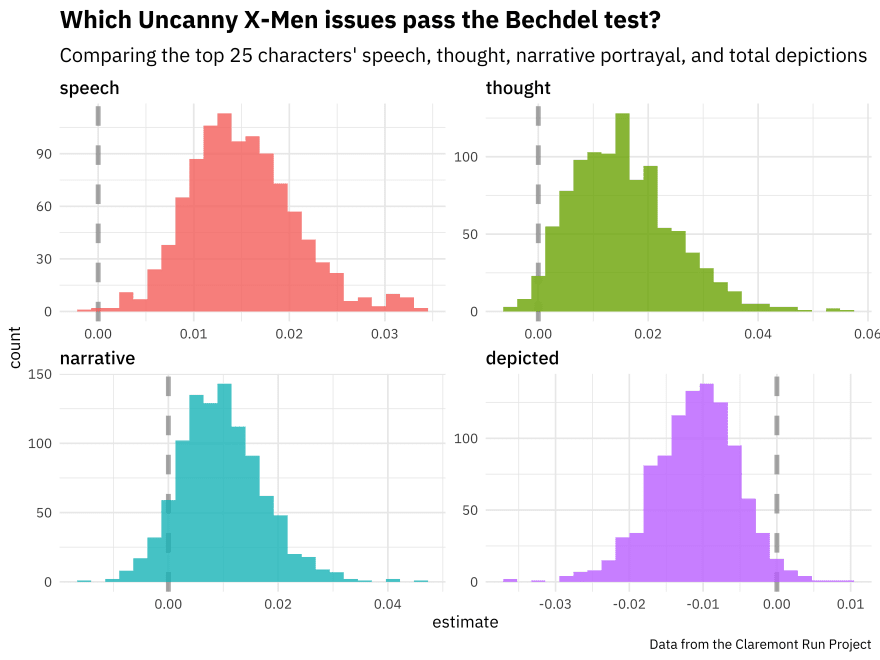
- Issues with more depictions of the main 25 characters (i.e. more characters in them) are less likely to pass the Bechdel test.
- Issues with more speech bubbles from these characters are more likely to pass the Bechdel test. (Perhaps also issues with more thought bubbles.)
I think it makes sense that issues with lots of speaking are more likely to pass the Bechdel test, which is about characters speaking to each other. Interesting that the issues with lots of character depictions are less likely to pass!

Oldest comments (0)