
This is the latest in my series of screencasts, but instead of being about tidymodels, this screencast focuses on unsupervised modeling for text, specifically topic modeling. Today’s screencast walks through how to build a structural topic model and then how to explore and understand it, with this week’s #TidyTuesday dataset on Spice Girls lyrics. 👯♀️
Here is the code I used in the video, for those who prefer reading instead of or in addition to video.
Explore data
Our modeling goal is to “discover” topics in the lyrics of Spice Girls songs. Instead of a supervised or predictive model where our observations have labels, this is an unsupervised approach.
library(tidyverse)

lyrics <- read_csv("https://raw.githubusercontent.com/rfordatascience/tidytuesday/master/data/2021/2021-12-14/lyrics.csv")
How many albums and songs are there in this dataset?
lyrics %>% distinct(album_name)


## # A tibble: 3 × 1
## album_name
## <chr>
## 1 Spice
## 2 Spiceworld
## 3 Forever


lyrics %>% distinct(album_name, song_name)


## # A tibble: 31 × 2
## album_name song_name
## <chr> <chr>
## 1 Spice "Wannabe"
## 2 Spice "Say You\x92ll Be There"
## 3 Spice "2 Become 1"
## 4 Spice "Love Thing"
## 5 Spice "Last Time Lover"
## 6 Spice "Mama"
## 7 Spice "Who Do You Think You Are"
## 8 Spice "Something Kinda Funny"
## 9 Spice "Naked"
## 10 Spice "If U Can\x92t Dance"
## # … with 21 more rows
Let’s start by tokenizing this text and removing a small set of stop words (as well as fixing that punctuation).
library(tidytext)

tidy_lyrics <-
  lyrics %>%
  mutate(song_name = str_replace_all(song_name, "\x92", "'")) %>%
  unnest_tokens(word, line) %>%
  anti_join(get_stopwords())
What are the most common words in these songs after removing stop words?
tidy_lyrics %>%
  count(word, sort = TRUE)


## # A tibble: 979 × 2
## word n
## <chr> <int>
## 1 get 153
## 2 love 137
## 3 know 124
## 4 time 106
## 5 wanna 102
## 6 never 101
## 7 oh 88
## 8 yeah 88
## 9 la 85
## 10 got 82
## # … with 969 more rows
How about per song?
tidy_lyrics %>%
  count(song_name, word, sort = TRUE)


## # A tibble: 2,206 × 3
## song_name word n
## <chr> <chr> <int>
## 1 Saturday Night Divas get 91
## 2 Spice Up Your Life la 64
## 3 If U Can't Dance dance 60
## 4 Holler holler 48
## 5 Never Give Up on the Good Times never 47
## 6 Move Over generation 41
## 7 Saturday Night Divas deeper 41
## 8 Move Over yeah 39
## 9 Something Kinda Funny got 39
## 10 Never Give Up on the Good Times give 38
## # … with 2,196 more rows
This gives us an idea of how many counts per words we have per song, for our modeling.
Train a topic model
To train a topic model with the stm package, we need to create a sparse matrix from our tidy dataframe of tokens.
lyrics_sparse <-
  tidy_lyrics %>%
  count(song_name, word) %>%
  cast_sparse(song_name, word, n)

dim(lyrics_sparse)


## [1] 31 979
This means there are songs (i.e. documents) and 979 different tokens (i.e. terms or words) in our dataset for modeling.
A topic model like this one models:
- each document as a mixture of topics
- each topic as a mixture of words
The most important parameter when training a topic modeling is K, the number of topics. This is like k in k-means in that it is a hyperparamter of the model and we must choose this value ahead of time. We could try multiple different values to find the best value for K, but this is a very small dataset so let’s just stick with K = 4.
library(stm)
set.seed(123)
topic_model <- stm(lyrics_sparse, K = 4, verbose = FALSE)
To get a quick view of the results, we can use summary().
summary(topic_model)


## A topic model with 4 topics, 31 documents and a 979 word dictionary.

## Topic 1 Top Words:
## Highest Prob: get, wanna, time, night, right, deeper, come
## FREX: deeper, saturday, comin, get, lover, night, last
## Lift: achieve, saying, tonight, another, anyway, blameless, breaking
## Score: deeper, saturday, lover, get, wanna, night, comin
## Topic 2 Top Words:
## Highest Prob: dance, yeah, generation, know, next, love, naked
## FREX: next, naked, denying, foolin, nobody, wants, meant
## Lift: admit, bein, check, d'ya, defeat, else, foolin
## Score: next, naked, dance, generation, denying, foolin, nobody
## Topic 3 Top Words:
## Highest Prob: got, holler, make, love, oh, something, play
## FREX: holler, kinda, swing, funny, yay, use, trust
## Lift: anyone, bottom, driving, fantasy, follow, hoo, long
## Score: holler, swing, kinda, funny, yay, driving, loving
## Topic 4 Top Words:
## Highest Prob: la, never, love, give, time, know, way
## FREX: times, tried, swear, la, bring, promise, viva
## Lift: able, certain, love's, rely, affection, shy, replace
## Score: la, times, swear, shake, viva, chicas, front
Explore topic model results
To explore more deeply, we can tidy() the topic model results to get a dataframe that we can compute on. There are two possible outputs for this topic model, the "beta" matrix of topic-word probabilities and the "gamma" matrix of document-topic probabilities. Let’s start with the first.
word_topics <- tidy(topic_model, matrix = "beta")
word_topics


## # A tibble: 3,916 × 3
## topic term beta
## <int> <chr> <dbl>
## 1 1 achieve 1.66e- 3
## 2 2 achieve 2.14e-21
## 3 3 achieve 1.75e-49
## 4 4 achieve 5.18e-36
## 5 1 baby 1.20e- 2
## 6 2 baby 1.44e- 2
## 7 3 baby 1.29e-15
## 8 4 baby 5.04e- 3
## 9 1 back 1.94e- 2
## 10 2 back 5.49e- 4
## # … with 3,906 more rows
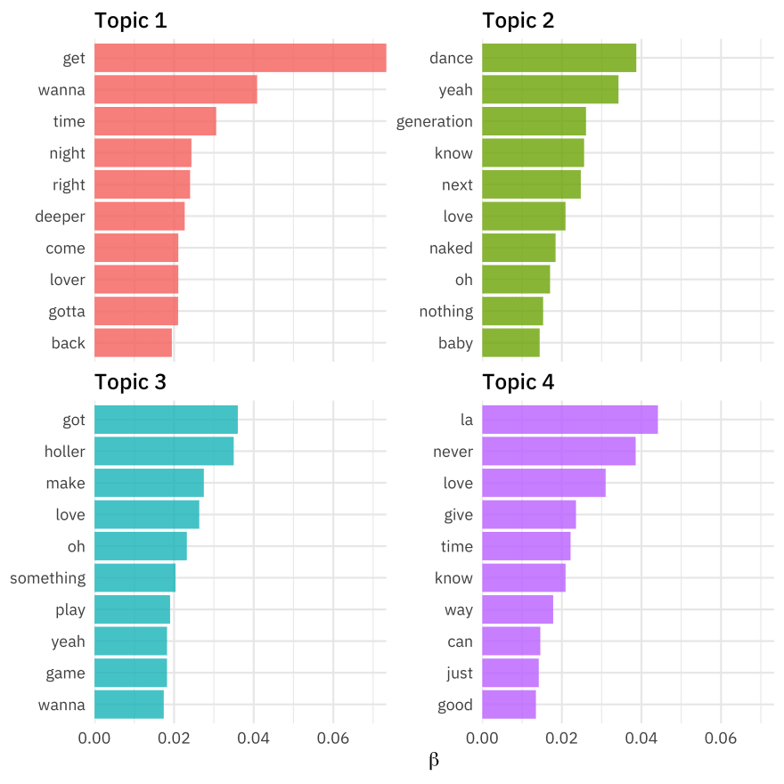
Since this is a tidy dataframe, we can manipulate it how we like, include making a visualization showing the highest probability words from each topic.
word_topics %>%
  group_by(topic) %>%
  slice_max(beta, n = 10) %>%
  ungroup() %>%
  mutate(topic = paste("Topic", topic)) %>%
  ggplot(aes(beta, reorder_within(term, beta, topic), fill = topic)) +
  geom_col(show.legend = FALSE) +
  facet_wrap(vars(topic), scales = "free_y") +
  scale_x_continuous(expand = c(0, 0)) +
  scale_y_reordered() +
  labs(x = expression(beta), y = NULL)
What about the other matrix? We also need to pass in the document_names.
song_topics <- tidy(topic_model,
  matrix = "gamma",
  document_names = rownames(lyrics_sparse)
)
song_topics


## # A tibble: 124 × 3
## document topic gamma
## <chr> <int> <dbl>
## 1 2 Become 1 1 0.714
## 2 Denying 1 0.00163
## 3 Do It 1 0.996
## 4 Get Down With Me 1 0.947
## 5 Goodbye 1 0.00106
## 6 Holler 1 0.00103
## 7 If U Can't Dance 1 0.000942
## 8 If You Wanna Have Some Fun 1 0.00722
## 9 Last Time Lover 1 0.998
## 10 Let Love Lead the Way 1 0.00175
## # … with 114 more rows
Remember that each document (song) was modeled as a mixture of topics. How did that turn out?
song_topics %>%
  mutate(
    song_name = fct_reorder(document, gamma),
    topic = factor(topic)
  ) %>%
  ggplot(aes(gamma, topic, fill = topic)) +
  geom_col(show.legend = FALSE) +
  facet_wrap(vars(song_name), ncol = 4) +
  scale_x_continuous(expand = c(0, 0)) +
  labs(x = expression(gamma), y = "Topic")
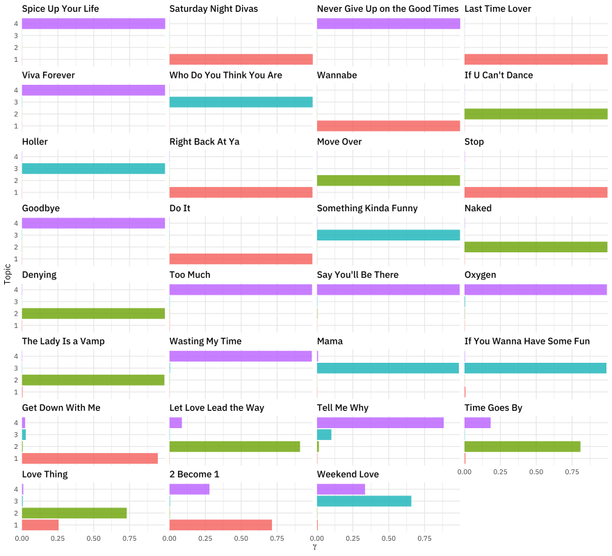
The songs near the top of this plot are mostly one topic, while the songs near the bottom are more a mix.
There is a TON more you can do with topic models. For example, we can take the trained topic model and, using some supplementary metadata on our documents, estimate regressions for the proportion of each document about a topic with the metadata as the predictors. For example, let’s estimate regressions for our four topics with the album name as the predictor. This asks the question, “Do the topics in Spice Girls songs change across albums?”
effects <-
  estimateEffect(
    1:4 ~ album_name,
    topic_model,
    tidy_lyrics %>% distinct(song_name, album_name) %>% arrange(song_name)
  )
Again, to get a quick view of the results, we can use summary(), but to dive deeper, we will want to use tidy().
summary(effects)


##
## Call:
## estimateEffect(formula = 1:4 ~ album_name, stmobj = topic_model,
## metadata = tidy_lyrics %>% distinct(song_name, album_name) %>%
## arrange(song_name))
##
##
## Topic 1:
##
## Coefficients:
## Estimate Std. Error t value Pr(>|t|)
## (Intercept) 0.1787 0.1312 1.362 0.184
## album_nameSpice 0.1199 0.1892 0.634 0.531
## album_nameSpiceworld 0.1139 0.1862 0.612 0.546
##
##
## Topic 2:
##
## Coefficients:
## Estimate Std. Error t value Pr(>|t|)
## (Intercept) 0.1444 0.1325 1.090 0.285
## album_nameSpice 0.1357 0.1879 0.722 0.476
## album_nameSpiceworld 0.1486 0.1846 0.805 0.427
##
##
## Topic 3:
##
## Coefficients:
## Estimate Std. Error t value Pr(>|t|)
## (Intercept) 0.27150 0.12085 2.247 0.0327 *
## album_nameSpice 0.01954 0.16752 0.117 0.9080
## album_nameSpiceworld -0.25776 0.16700 -1.543 0.1339
## ---
## Signif. codes: 0 ' ***' 0.001 '**' 0.01 '*' 0.05 '.' 0.1 ' ' 1
##
##
## Topic 4:
##
## Coefficients:
## Estimate Std. Error t value Pr(>|t|)
## (Intercept) 0.405559 0.140820 2.880 0.00754 **
## album_nameSpice -0.273207 0.202200 -1.351 0.18746
## album_nameSpiceworld -0.007134 0.194246 -0.037 0.97096
## ---
## Signif. codes: 0 ' ***' 0.001 '**' 0.01 '*' 0.05 '.' 0.1 ' ' 1


tidy(effects)


## # A tibble: 12 × 6
## topic term estimate std.error statistic p.value
## <int> <chr> <dbl> <dbl> <dbl> <dbl>
## 1 1 (Intercept) 0.177 0.132 1.34 0.190
## 2 1 album_nameSpice 0.120 0.189 0.633 0.532
## 3 1 album_nameSpiceworld 0.115 0.188 0.608 0.548
## 4 2 (Intercept) 0.145 0.133 1.09 0.283
## 5 2 album_nameSpice 0.135 0.187 0.722 0.476
## 6 2 album_nameSpiceworld 0.150 0.185 0.813 0.423
## 7 3 (Intercept) 0.272 0.120 2.26 0.0316
## 8 3 album_nameSpice 0.0167 0.167 0.100 0.921
## 9 3 album_nameSpiceworld -0.259 0.166 -1.57 0.129
## 10 4 (Intercept) 0.404 0.140 2.89 0.00739
## 11 4 album_nameSpice -0.273 0.196 -1.39 0.175
## 12 4 album_nameSpiceworld -0.00502 0.193 -0.0260 0.979
Looks like there is no statistical evidence of change in the lyrical content of the Spice Girls songs across these three albums!

Latest comments (0)