Let's say you have an array and you need to come up with a function that checks if the array has a given number n.
You then write a simple function such as this:
const linearSearch = (array, n) => {
  for(let i = 0; i < array.length; i++) {
    if(array[i] == n) {
      return console.log(`${n} is at index ${i}`)
    }
  }
  return console.log(`${n} not found`);
}
...and you are done or are you?
Well, you might be in the best-case scenario where the given array is small enough and the function executes swiftly.
But life ain't always that easy!
What if the given array is huge? And, say, n is not equal to the first element in the array but somewhere in the middle or not even there? The linear search function we wrote above still works but what about the execution time to go over each element in the array until it comes across the element we are looking for?

Make it work. Make it right. Make it fast!
Following this cliched mantra for programmers, one should really consider the different scenarios -- the best, the worst and the acceptable one, before implementing algorithms.
That's when the Big O comes into play.

Big O notation in Computer Science is used to explain how the runtime or the space used scales with respect to input variable(s) and is essential in understanding the efficiency of an algorithm. In this post, I will mostly focus on the time complexity so let's go over some common runtimes.
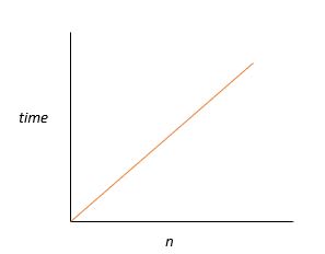
O(N) - Linear
O(N) describes the performance of an algorithm that scales linearly with the input size. Say, you have an array of 100 element. It would take 100 iterations through the loop to console.log() all the items. Similarly, with one million elements it would take one million iterations. Hence, the time complexity is directly proportional to the data input size.
O(1) - Constant Time Complexity
With constant time complexity, the time taken to execute is constant regardless of the size of the data input. Let's say you have a file to transfer over from one city to another. Normally, you'd attach the file to an email and send it over or decide to do a FTP transfer. In either case, the bigger the file size, the longer it would take for you to transfer the file over. Hence, the runtime would be linear, i.e. O(N).
However, let's say you come up with an ingenious idea of transferring your gigantic file to a flash drive and sending it over to the recipient via a pigeon (because mailing is boring) that you trained to do so. Now, think about the relationship between the file size and the transfer time. Would it matter if the file was 1GB or 1TB? Our pigeon friend would still take the same amount of time to fly over and deliver the flash drive. So, here our runtime would be O(1), meaning our algorithm will always execute at the same time regardless of the size of the input data. In that case a pigeon would be faster than the internet.

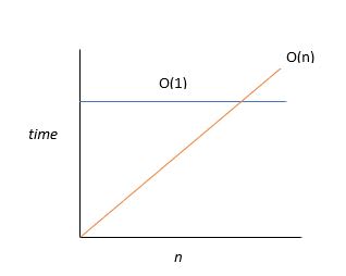
It's not to say that O(1) is always better than O(N) or vice versa. It really depends on the size of the input variable. The figure below demonstrates how at some point O(N) algorithm will surpass the runtime of an O(1) algorithm, thereby making O(1) a better choice for data of the size that is greater than that which corresponds to the interception point. However, prior to the interception point, O(N) is more efficient.
O(N^2) - Quadratic
O(N^2) describes an algorithm whose performance is directly proportional to the square of the size of the input data set. This commonly involves nested iterations over the data set, like:
let arr = [1,2,3,4,5];

for(let i = 0; i < arr.length; i++) {
  for(let j = 0; j < arr.length; j++) {
    console.log(i +"" +j);
  }
}
Some other examples would be bubble sort and comparing elements in two arrays of the same size.
O(2^N)
Another common runtime you might see is O(2^N). Algorithms with this runtime are often recursive algorithms that solve a problem of size N by recursively solving two smaller problems of size N-1. The growth curve of an O(2^N) function is exponential - starting off very shallow, then rising sharply.

A good example of O(2^N) algorithm is the recursive calculation of Fibonacci number.
function calculateFibonacciNumber(N) {
  if (N <= 1) {
     return N;
  } else {
   return calculateFibonacciNumber(N - 2) + calculateFibonacciNumber(N - 1);
}
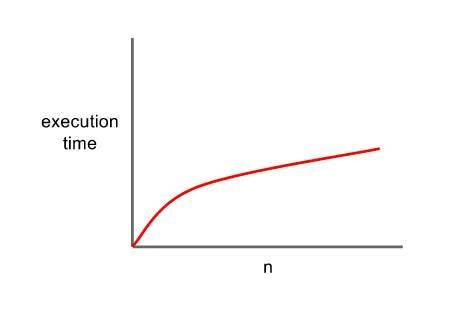
O(logN) - Logarithmic
With logarithmic notation execution time increases, but at a decreasing rate. Performing Binary Search on a sorted array is a good example of O(logN) runtime. Such algorithm traverses the input data once and then on every subsequent iteration the size of the input data is halved. Below is the growth curve depicting a logarithmic runtime. You can tell why Binary Search is a good choice when it comes to working with a large data.
Note:
There are couple of things to note while calculating Big O notation.
1) Drop the constant and the non-dominant terms
Big O takes the worst case into consideration so we are trying to predict what happens to our algorithm's efficiency when the data input size is ridiculously big. In that sense, if N's value is ridiculously huge, any other constant compares almost non-existent to N. Hence, we drop the constants. So, O(2N) is simply O(N). Likewise, we also drop the non-dominant terms. For instance, O(N^2 + N) becomes O(N^2), O(N+logN) becomes O(N) and so on.
2) Multiply v. Add
If we do A chunks of work then B chunks of work, the total amount of work is O(A+B)
arrayA.forEach(el => console.log(el))
Similarly, if we do B chunks of work for each element in A, the total amount of work is O(AxB)
arrayA.forEach ( a => {
   arrayB.forEach ( b => {
    console.log(a+" " + b);
   })
})
And, finally here's a graph I pulled from this post showing how different runtimes compare.

Conclusion
If you are new to programming, Big O notation might not be your primary focus. However, as you embark on your journey to becoming an awesome programmer you will want to understand the complexities of your algorithms and how they will behave when the input size grows. This is the real world we are talking about and you never know what size of data you might have to work with. Hence, Big O lets us prepare ourselves for the worst-case scenarios, helping us make a sound decision when it comes to devising and implementing algorithms.

Top comments (0)