Monitoring data drift in machine learning models

Data drift is a phenomenon in which the input variables of a model change their usual behavior, leading to a decrease in model performance. Therefore, creating processes to monitor potential changes in the population is crucial when deploying a model in a production environment.

In the following documentation, an automated workflow is developed using step functions, implementing a solution that compares the distributions of each variable using the non-parametric Kolmogorov-Smirnov statistical test between the original dataset and the new data sample. If a statistical variation is found in at least one variable, the model will be updated by retraining the algorithm, followed by generating new predictions through a batch process.

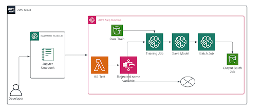
Architecture diagram

AWS services are used for what purposes in this architecture:

Sagemaker StudioLab: It is used to test the code to be executed and perform testing.

Step Functions: It will be our conductor, indicating step by step how the flow should proceed.

SageMaker: It will handle our machine learning-related jobs; it is the service par excellence for this purpose. It offers a wide range of instances that will adjust to the exact requirement.

S3 Bucket: It is used to retrieve the training data and then store the batch results.

Lambda: It is used to perform the test, and its output will be our variable for comparison.

First Step:

1- Associate accounts: Our first step will always be to be aware of the roles we will need to execute tasks related to the processes. Therefore, it is vital to have an AWS account in order to provide the necessary roles to the notebook.

2- Load Amazon Sagemaker Studio Labs libraries: Among the modules to be imported, our main development tool is the Step Functions Data Science SDK. It will allow us to create the entire flow within our notebook.

3- Lambda function creation: A lambda function is created to apply the Kolmogorov-Smirnov (K-S) statistical test, a non-parametric test that aims to test the hypothesis that two probability distributions are identical or different. The implemented function performs a hypothesis test on each pair of variables associated with the dataset used to train the model and the dataset with new collected samples. The K-S test is already implemented in the Python module Scipy.

import json
import boto3
import csv
from io import TextIOWrapper
import urllib3
import random
import pandas as pd
import scipy
import io
from scipy import stats


def lambda_handler(event, context):
    bucket='yourbucket-name'
    key='new-data.csv'
    s3 = boto3.client('s3')
    response = s3.get_object(Bucket=bucket, Key=key)   #["Body"].read()
    chunks = (chunk for chunk in response["Body"].iter_chunks(chunk_size=1024**3))
    data = io.BytesIO(b"".join(chunks)) # This keeps everything fully in memory
    df_new = pd.read_csv(data) # here you can provide also some necessary args and kwargs

    ## la otra data 

    key2='current-data.csv'
    response2 = s3.get_object(Bucket=bucket, Key=key2)
    chunks2 = (chunk for chunk in response2["Body"].iter_chunks(chunk_size=1024**3))
    data2 = io.BytesIO(b"".join(chunks2))
    df2 = pd.read_csv(data2)

    # entra scipy en acción
    p_value = 0.05
    rejected = 0
    numerical=df_new.iloc[:,1:] #take columns and discard target

    for col in numerical.columns:
        test = stats.ks_2samp(df_new[col], df2[col])
        if test[1] < p_value:
            rejected += 1
            print("Column rejected", col)
            print("We rejected",rejected,"columns in total")

    return (rejected)

4- Training configuration: The parameters for executing the training are set from the notebook, which helps us develop an optimal model. This work will ultimately be executed from AWS, using a machine optimized for machine learning.

5- Flow definition: Once each step of our flow is configured, we generate a pipeline for each stage using a step function. The chain of processes begins by applying the K-S test, as explained earlier. If there is one or more rejected hypothesis tests, the model update process will be initiated, starting with training and followed by a batch inference job.

6- Step Functions flow deployment: Finally, the flow is deployed, where one of the variables has a different distribution compared to the initial dataset, resulting in a rejection in the hypothesis test of the variable. This triggers the corresponding processes in the pipeline illustrated in the figure.

Conclusion

In this exercise, a tool was successfully implemented to monitor possible changes in the population, enabling automated retraining of a new model to ensure accurate predictions. The main development involved constructing a Lambda function and adding the necessary configurations to perform statistical tests. Along the same line, a next step is to incorporate other tools to handle data drift, such as the concept of Population Stability Index (PSI).