
In Part 2 of this series I introduced graphs. A graph is a representation of connections between nodes in a network. The connections between the nodes are called 'edges'. For example, in a geographical network nodes might be towns and edges might be the roads that connect the towns.
I also introduced you to the breadth-first search ("BFS") algorithm: a means to find the shortest route through a graph. In the context of BFS, shortest route means the route that visits the fewest nodes. In this article I will add a little complexity to graphs by adding "weights" and introduce Dijkstra's Algorithm which will find the shortest route through these more complex weighted graphs.
Weighted graphs
Imagine a graph with nodes representing cities (Manchester, Birmingham, Milton Keynes, London & Edinburgh) and the edges between them representing railway tracks.
Here is a picture of that graph.
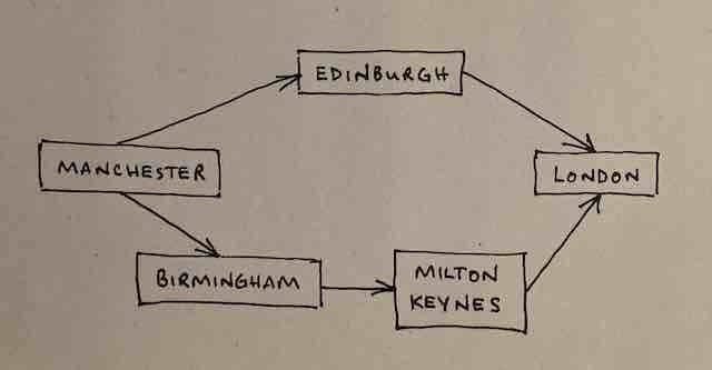
You want to get from Manchester to London by train. Which route should you take? Well, we know that BFS will find the shortest path so we feed the graph into the algorithm, set it running, and it confidently tells us to go via Edinburgh.
Ok, that's the route to take if you want the fewest stops - which is what BFS tells you - in the context of BFS, shortest route means the route that visits the fewest nodes.
Let's add distances between cities:

Now we can see quite clearly what we already knew: the shortest route is via Birmingham & Milton Keynes at 200 miles rather than the 610 miles via Edinburgh.
In graph terminology the numbers that represent the distance between nodes are the weights of those edges. Weights don't have to represent distance. It could represent the cost of getting from one node to the next, for example.
If you want to find the shortest path in a weighted graph, BFS simply won't cut the mustard. You need another graph algorithm: you need Dijkstra's algorithm, named after computer scientist Edsger Dijkstra who conceived of the idea about 65 years ago.
Dijkstra's will find the cheapest / shortest path (in other words, the one with the lowest combined edge weights) in a weighted graph.
For example:
nodes on a geographical graph - Dijkstra's will find the shortest route, like the example above.
nodes in a graph of transactions - Dijkstra's will find the lowest cost chain of transactions.
Dijkstra's - the steps
- Set up a list of all nodes. The list will hold the cumulative weight of getting to that node. If you can't yet calculate the cumulative weight because your route hasn't yet reached that node, give it a cumulative weight of positive infinity (this may sound odd but it's an integral part of the algorithm's workings)
- From the current node, find the lowest cost node. ie. the node you get to by following the lowest weight edge
- For all neighbours of that node check if there is a lower cumulative-weight way to get there. If so, update that node's cumulative weight in the list that you set up at the outset. (Remember, any nodes where you can't calculate the cumulative weight from the current node have an infinite cumulative weight)
- Repeat until you have done this for every node in the graph.
- Then calculate the final path.
Clarification of the values that are being recorded here
In the steps above you will notice that there are two different weight-related values. It's worth spending a moment to think those values through.
Edge weights - this is the "cost" of travelling from one node to another along that particular edge. An edge's weight is a fixed value: it never changes throughout the progress of the algorithm.
Node cumulative weights - these are the values held in the list that was set up at the start. For a given node, this is the cumulative weight of all of the edges along which you have to travel to get to a specific node if you follow the lowest cost route that the algorithm has calculated so far. These values are updated as the algorithm processes the nodes in the graph.
Dijkstra's - initial setup
We need a graph to work with. Here is a simple example that the remainder of this article will refer to:

As we discovered with BFS, setting up the required data structures represents a significant part of the work in graph algorithms.
The graph
First we need a hash table to represent the graph. In BFS each node was a key in the hash table and its value was an array of the node's neighbours. The graph we are building here has an extra data point for every connection: the weight of the edge. To cater for that each node in the hash table will hold its own hash table (as opposed to the simple array in BFS).
The slightly confusing explanation in that previous paragraph will hopefully become clearer when you look at the code below. Again I am using JavaScript's Map() object as a hash table.
const graph = new Map();
graph.set("start", new Map());
graph.get("start").set("a", 6);
graph.get("start").set("b", 2);
graph.set("a", new Map());
graph.get("a").set("fin", 1);
graph.set("b", new Map());
graph.get("b").set("a", 3);
graph.get("b").set("fin", 5);
graph.set("fin", new Map());
Cumulative node weights
Next we need a structure to keep track of the cumulative weight of every node. Again a Map() is the perfect data structure:
costs.set("a", 6);
costs.set("b", 2);
costs.set("fin", Number.POSITIVE_INFINITY);
Notice how the "fin" node has a cumulative cost of POSITIVE_INFINITY (a JavaScript constant). From the start node, we can't "see" the route to the finish node - all we know is that going to A "costs" 6 and going to B "costs" 2. Remember, any nodes where you can't calculate the cumulative weight from the current node have an infinite cumulative weight.
Parents
There is one data requirement that hasn't been mentioned yet. As the algorithm traces its way through the graph, plotting the "lowest cost" route, we need to keep track of that route. Dijkstra's does that by, for every node, keeping track of the previous node in the path. So every node (apart from the start node) will have a "parent" node.
Every node's parent is recorded in a parents hash table (or Map() in JavaScript). At the outset it looks like this:
const parents = new Map();
parents.set("a", "start");
parents.set("b", "start");
parents.set("fin", null);
Every time a node's cumulative weight is updated (because a lower cost path has been found) the parent for that node also needs to be updated.
Notice that the "fin" node's parent starts out having a null value. That's because we won't know that node's parent until the routing process has got that far.
Processed nodes
And the last part of the data structure setup - to avoid loops we need to keep track of nodes already visited. That just takes the form of an array called processed.
const processed = [];
Processing the graph
Now that we have the initial data structures set up we can start processing the graph.
Lowest cost node
The first activity on arriving at a new node is to find the lowest cost node that hasn't already been processed because that node will be the next one to visit. Remember that all nodes (apart from immediate neighbours of start) were initially assigned a cumulative weight of infinity and those figures are only updated as we visit their neighbours. So, ignoring nodes that have already been processed (held in the processed array), the lowest cost node will automatically be a neighbour of the node we are currently processing and we just need to loop through all nodes in the costs hash table and do a comparison.
The findLowestCostNode() function looks like this:
function findLowestCostNode(costs) {
  lowestCost = Number.POSITIVE_INFINITY;
  lowestCostNode = null;
  costs.forEach((cost, node) => {
    if (cost < lowestCost && !processed.includes(node)) {
      lowestCost = cost;
      lowestCostNode = node;
    }
  });
  return lowestCostNode;
}
Graph traversal
We have set up the data structures and we have a function to decide which node to visit next. Now we just need to loop through the nodes and carry out the steps outlined above. Below is the code that achieves that:
let node = findLowestCostNode(costs);
while (node) {
  const nodeCost = costs.get(node);
  const neighbours = graph.get(node);
  neighbours.forEach((cost, neighbour) => {
    newNodeCost = nodeCost + cost;
    if (costs.get(neighbour) > newNodeCost) {
      costs.set(neighbour, newNodeCost);
      parents.set(neighbour, node);
    }
  });
  processed.push(node);
  node = findLowestCostNode(costs);
}
We have to define the first lowest cost node (ie. a neighbour of the start node) before entering the while loop because 'node' being truthy is the while loop condition. The lowest cost node is then updated at the end of each iteration until there are no nodes left to process.
After the algorithm has finished processing the graph, the value of the "fin" node in the costs hash table will contain the cumulative cost of the lowest cost path. (In this case: 6)
console.log(costs.get("fin")); // 6
To find the actual path that the algorithm has plotted you need to begin with the end node and work backwards using the values in the parents hash table. In this simple example, the parents hash table looks like this after processing:
{ 'a' => 'b', 'b' => 'start', 'fin' => 'a' }
So, working backwards:
- from
fingo toa - from
ago tob - from
bgo tostart
There you have the lowest cost route.
Larger example
It's fair to say that the graph we are working with here is trivially small. I am able to confirm however that the method does work on more complex graphs. Take a look at this problem: Part 1 of Day 15 of the 2021 Advent of Code.
The graph in this problem is a 100 x 100 matrix of digits (available here). Your job is to find the lowest cost route from top-left to bottom-right through the matrix, moving one node at a time up, down, left or right, where the cost increases by the value of each node visited.
Here is my code to solve the problem. The first ~half of the code builds the graph hash map and the other data structures that are discussed in this article. The rest of the code is essentially the function and while loop shown above.
On my ~9 year old Mac it took about 13 minutes to come up with the lowest cost route. I dare say there is a more efficient and/or elegant approach but the fact that it provided the correct answer is evidence that the algorithm does work with larger, more complex graphs.
If you want to give it a whirl the correct answer is shown in a comment at the bottom of the file on GitHub.
Summary
In this article I have dug a little deeper into graphs and added weights to the edges. I have also taken you step by step through Dijkstra's algorithm to find the lowest cost route through a weighted graph.
You have also learned how to put together the code that will carry out Dijkstra's algorithm.
The next, and final, part in this series will look at dynamic programming algorithms and how to use one to solve the Knapsack Problem.
Cover image by Gene Jeter on Unsplash

Top comments (0)