Understanding vector search and HNSW index with pgvector

Vector embeddings have become an essential component of Generative AI applications. These embeddings encapsulate the meaning of the text, thus enabling AI models to understand which texts are semantically similar. The process of extracting the most similar texts from your database to a user’s request is known as nearest neighbors or vector search.

pgvector is the Postgres extension that allows vector search. The latest release of pgvector 0.5.0 includes a new graph-based index for approximate nearest neighbor (ANN) search known as Hierarchical Navigable Small Worlds (HNSW). This new index makes vector search queries significantly faster and your AI applications more responsive. But what does this mean for developers and Large Language Model (LLM) applications?

In this article, we will explore:

1. What vector similarity search is
2. Why do you use vector search for LLM apps
3. How to optimize vector search with approximate nearest neighbor algorithms

Vectors and Vector Embeddings

What are Vectors?

In simple terms, a vector is a list of numbers that can represent a point in space. For example, in 2D space, a vector [2,3] represents a point that’s 2 units along the x-axis and 3 units along the y-axis. In 3D space, a vector [2,3,4] adds an additional dimension, the z-axis. The beauty of vectors is that they can have many more dimensions than we can visualize.

Vector Embeddings

The word “embedding” might sound complex, but it’s just a fancy way of saying “representation.” When we say “vector embeddings,” we’re referring to representing complex data, like words or images, as vectors.

Cat: [0.8108,0.6671,0.5565,0.5449,0.4466]

For example, consider the word “cat.” Instead of thinking about it as a string of letters, we can represent it as a point in a multi-dimensional space using a vector. This representation can capture the essence or meaning of the word in relation to other words. Words with similar meanings would be closer in this space, while different ones would be further apart.

Why use Vector Embeddings?

Vector embeddings allow us to convert diverse forms of data into a common format (vectors) that LLMs can understand and process. By doing so, we can perform mathematical operations on them, like calculating the distance between two vectors, which can tell us how similar or different two pieces of data are.

​​Similarity Search

Imagine you have a specific song stuck in your head, but you don’t know its title. Instead of listening to each song in a vast playlist, you’d want to find the one that closely matches the tune or lyrics you remember. In the world of vectors, this is called “similarity search.”

When we represent data as vectors, we can measure how close or far apart these vectors are. Let’s assume we have the words apple, cat and dog represented by 5-dimension vector embeddings.

Apple: [−0.7888,−0.7361,−0.6208,−0.5134,−0.4044]
Cat: [0.8108,0.6671,0.5565,0.5449,0.4466]
Dog: [0.8308,0.6805,0.5598,0.5184,0.3940]">

Now, we want to know which word is the closest semantically to the word orange.

Orange: [−0.7715,−0.7300,−0.5986,−0.4908,−0.4454]

The orange vector here is called the query vector. We know that orange is a fruit, so logically it can be grouped with the word apple. Let’s visualize our vectors on a two-dimensional plane. We can reduce the 5-dimensional vectors to 2-dimensional ones for visualization through Principle Component Analysis.

We can observe that we have two clusters: animals and fruit. The closer two vectors are, the more similar the data they represent is. So, to perform a similarity search, we need to calculate the distance between the query vector (orange) and all our vectors (cat, dog, apple) and find out which one is the smallest. Next, we’ll see how to calculate the distance between two vectors.

Distance metrics

The concept of “distance” between vectors is pivotal in similarity search. There are various ways to measure this distance, the most common being the Euclidean distance. However, the cosine similarity often proves more effective for high-dimensional data (like text or images).

Eucledian or L2 distance

The L2 distance, also known as Euclidean distance, is a measure of the straight-line distance between two points in Euclidean space. For two vectors A and B of length n, the L2 distance is calculated as follows:

Example:

Let’s say we have two vectors A=[1,2] and B=[2,2].

L2 Distance: D(A,B)=(1-2)2+(2-2)2​=1

In L2 distance metric, the smaller the distance_,_ the more similar A and B are. L2 performs well in use cases such as image recognition tasks where pixel-by-pixel differences are significant. However, unlike the Cosine distance function, L2 distances are always positive, which makes them less suitable for understanding dissimilarities.

Here is what the distances would look like using L2:

 | Apple | Orange | Cat | Dog |
---------------------------------------------------------------------------
Apple | 0.0 | 0.054965 | 2.785305 | 2.779520 |
Orange | 0.054965 | 0.0 | 2.767337 | 2.760769 |
Cat | 2.785305 | 2.767337 | 0.0 | 0.063714 |
Dog | 2.779520 | 2.760769 | 0.063714 | 0.0 |">

Cosine distance

Cosine distance is a measure of similarity derived from the cosine similarity metric. It’s often used for document retrieval use cases where the angle between vectors identifies the similarity in content.

While cosine similarity measures the cosine of the angle between two vectors, cosine distance is defined as the complement to cosine similarity, and is calculated as:

Cosine distance ranges from 0 to 2, where 0 indicates that the vectors are identical, and 2 indicates that they are diametrically opposed.

Example

For the same A=[1,2] and B=[2,2].

1. Calculate the Dot Product: A⋅B=(1×2)+(2×2)=2+4=6

2. Calculate the Magnitude: A= 12+22​ =5​ , B= 22+22​ =8​

3. Calculate the Cosine Distance: _D(A,B)=1− 65 8​ 0.0513 _

The matrix below shows the distances for our vectors:

 | Apple | Orange | Cat | Dog |
---------------------------------------------------------------------------
Apple | 0.0 | 0.000689 | 1.997025 | 1.997994 |
Orange | 0.000689 | 0.0 | 1.997349 | 1.997192 |
Cat | 1.997025 | 1.997349 | 0.0 | 0.001058 |
Dog | 1.997994 | 1.997192 | 0.001058 | 0.0 |">

Vector search with pgvector

pgvector is the Postgres extension for vector similarity search. Let’s see how to execute our previous example using pgvector:

CREATE EXTENSION vector;
-- Creating the table
CREATE TABLE words (
    word VARCHAR(50) PRIMARY KEY,
    embedding VECTOR(5)
);

-- Inserting the vectors
INSERT INTO words (word, embedding) VALUES
('Apple', '[-0.7888, -0.7361, -0.6208, -0.5134, -0.4044]'),
('Cat', '[0.8108, 0.6671, 0.5565, 0.5449, 0.4466]'),
('Dog', '[0.8308, 0.6805, 0.5598, 0.5184, 0.3940]');">

Here is an example of how to search vectors that are the closest to the word orange:

SELECT word FROM words
ORDER BY embedding <=> '[-0.7715, -0.7300, -0.5986, -0.4908, -0.4454]">

Output:

word  
-------
 Apple
 Dog
 Cat
(3 rows)">

The above query returns the list of word in the words table ordered by distance ascending order. The <=> operator is used for Cosine distances. pgvector supports many distance functions, including Cosine, L2 and Inner Product.

The above query returns all rows in the table words. Typically in real-world applications, we want to return the k most similar vectors.

SELECT word FROM words
ORDER BY embedding <=> '[-0.7715, -0.7300, -0.5986, -0.4908, -0.4454] LIMIT 1;">

Output:

word  
-------
 Apple
(1 row)">

The query above performs a sequential scan and compares all vectors with the query vector and returns id’s for the closest vector to our query vector. This method can be computationally costly with large datasets. In the next section, we will see how to optimize the vector similarity search with indexes.

Optimizing vector similarity search

In Postgres, an index sorts the table for efficient search. By default, pgvector performs a sequential scan and returns the vectors with 100% accuracy. We call this an exact search. This accuracy often comes at the expense of speed. Using approximate nearest neighbour (ANN) index search instead of exact search offers a significant advantage in terms of computational efficiency, especially at scale.

In an exact search, every query involves scanning the entire dataset to find the closest neighbors, leading to a time complexity of O(N), where N is the size of the dataset. This doesn’t scale well for large datasets and can be computationally expensive.

On the other hand, ANN algorithms like HNSW enable much faster queries by approximating the nearest neighbors. They do this by exploring a subset of the dataset, thereby reducing the computational burden.

While this comes at the cost of a slight reduction in the accuracy of the results, the trade-off is often acceptable for many real-world applications where speed is crucial. By enabling faster and more efficient queries, ANN search methods make it feasible to work with large-scale, high-dimensional data in real-time scenarios.

HNSW for ANN search

As you would have guessed by now, HNSW is an ANN index. Its graph-based nature is designed for efficient search, especially at larger scales. HNSW creates a multi-layered graph, where each layer represents a subset of the data, to quickly traverse these layers to find approximate nearest neighbors.

In each of the HNSW index layers, the vectors are sorted according to the distance function. The pgvector extension supports multiple distance functions. Next, we discuss the differences between those distances and which one you should choose for your application.

Now that we understand how vectors are sorted, let’s explore how HNSW connects vectors to each other to optimize for search.

Here is how you would create an HNSW index in Postgres:

CREATE INDEX ON words USING hnsw (embedding vector_cosine_ops) WITH (m = 10, ef_construction = 64);

The index build query above creates an HNSW index on the vectors column of documents table, using the cosine distance and the specified parameters m and ef_construction.

When you create an HNSW index, you’ll encounter two important parameters: m and ef_construction. These parameters control the index’s structure and impact both its build time and query performance.

m – The degree of the graph

The m parameter dictates how many connections (or “edges”) each data point (or “vertex”) has to its neighboring data points in the graph. For example, if m = 10, each data point in the graph would be connected to its four nearest neighbors.

Increasing m means that each point will be connected to more neighbors and would make the graph denser, which can speed up search queries at the cost of longer index build times and higher memory usage.

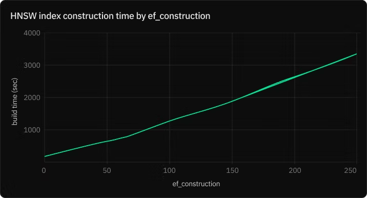
ef_construction – Candidate list size during index build

The ef_construction parameter controls the size of the candidate list used during the index building process. This list temporarily holds the closest candidates found so far as the algorithm traverses the graph. Once the traversal is done for a particular point, the list is sorted, and the top m closest points are retained as neighbors.

A higher ef_construction value allows the algorithm to consider more candidates, potentially improving the quality of the index. However, it also slows down the index building process, as more candidates mean more distance calculations.

Choosing the right values

In most cases, you’ll need to experiment to find the best values for your specific use case. However, general guidelines suggest:

– Smaller m values are better for lower-dimensional data or when you require lower recall.

– Larger m values are useful for higher-dimensional data or when high recall is important.

– Increasing ef_construction beyond a certain point offers diminishing returns on index quality but will continue to slow down index construction.

By understanding and carefully choosing these parameters, you can effectively balance the trade-offs between index quality, query speed, and resource usage.

Vector similarity search with HNSW

SET hnsw.ef\_search = 10;

SELECT word FROM words  
ORDER BY embedding <=> ‘[-0.7715, -0.7300, -0.5986, -0.4908, -0.4454]’ LIMIT 1;

The above query sets ef_search parameter and returns the query vectors k approximate nearest neighbors.

ef_search – Candidate list size during search

HNSW creates a hierarchical graph where each node is a vector, and edges connect nearby (similar) nodes. When searching for the nearest neighbors of a query vector, the algorithm navigates this graph. The parameter ef_search controls the size of the dynamic list used during the search process.

When you set ef_search, you’re specifying the size of the “beam” or the “priority queue” used during the search. It determines how many candidate vectors the algorithm will consider at each step while navigating the graph.

Trade-offs:

• Higher ef_search: Increases the search accuracy because the algorithm considers more candidate nodes. However, this also increases the search time since more nodes are being evaluated.
• Lower ef_search: Speeds up the search but might decrease accuracy. The algorithm might miss some closer nodes because it’s considering fewer candidates.

HNSW Pros and Cons

While speed with a high level of accuracy are the main advantage of HNSW, which helps Postgres-powered LLM applications scale to millions of users, the index is resource intensive. You would typically need more RAM and configure the maintenance_work_mem for larger datasets.

Advantages

• Speed : HNSW is significantly faster than traditional methods like IVF.
• High Recall : HNSW provides a high recall rate, meaning it’s more likely to return the most relevant results.
• Scalability : HNSW scales well with the size of the dataset.

Disadvantages

• Approximate Results : The algorithm provides approximate, not exact, results.
• Resource-Intensive Indexing : Creating an HNSW index can be resource-intensive, especially for large datasets.
• Complexity : The algorithm’s parameters can be tricky to tune for optimal performance.

Conclusion

Vectors have revolutionized how we handle and interpret data in AI. With pgvector and its integration of the HNSW algorithm in Postgres, developers now have an efficient tool to make AI applications even more responsive and accurate. While HNSW offers impressive speed, it’s essential to understand its trade-offs, especially when dealing with extensive datasets.

We genuinely hope pgvector becomes a valuable asset in your development toolkit. Your feedback is crucial for its continuous improvement. Enjoy exploring its capabilities and do share your experiences with us!