Unfolding a Machine Learning Classification Problem: A Step by Step Guide.

A classification problem in machine learning involves forecasting the class or category of an input sample based on its features or attributes. For instance, you want to build a machine learning model that can be able to distinguish a cat from a dog, the goal of this model will be to accurately predict the classes of new and unseen images of cats and dogs and assign each image its respective class. As such, this problem is classified as a classification problem.

Similar to other machine learning tasks, building a classification model involves a number of steps to achieve its primary objective. These steps include collecting and preprocessing the data, dividing it into training and testing sets, selecting a suitable model, training the model on the data, evaluating the performance of the model, optimizing the model, and finally deploying it in real-world applications such as web services, mobile apps, or APIs.

Some common applications of machine learning classification that you've probably interacted with include spam detection which I've just mentioned above, sentiment analysis, fraud detection, image classification, and medical diagnosis. This shows the classification technique have a wide pool of practical applications across various domains.

---

Types of Classification Approaches.

There exists three MAIN types of classification approaches, they include:

Binary Classification:

In binary classification, the goal is to classify instances into one of two classes or categories.These classes are assigned class labels - either 0 or 1. Class label 0 is mostly associated with the "normal state" of the category and vice versa.

Examples include a classifier determining if an email is spam or not, or if a person has a disease or not.

Some popular algorithms used in this type of classification problem include SGD classifier (very powerful esp when handling large datasets), K-Nearest Neighbors, and SVM.

Multi-class Classification:

In multiclass classification (also called multinomial classification), the goal is to classify instances into one of several possible classes or categories.

Examples include classifying images of animals into different types of species, or classifying news articles into different topics.

Random Forest and Naive Bayes classifiers usually perfom exceptionally well in this scenario. However, some binary classifiers such as SVM and Linear classifiers can also be used but in such a case, two strategies are used to train the classifier; either One-Versus-All or One-Versus-One.

Multi-label Classification:

On the other hand we have multi-label classification, whereby the goal is to assign one or more labels to each instance. This is different from multiclass classification, where each instance is assigned to only one class.

Examples include tagging documents with relevant keywords, or classifying images with multiple labels such as "sunset," "beach," and "ocean".

A common application of this is the face-recognition classifier which attaches a single tag per person in an image containing a number of people.

---

End-End Classification Task.

In this section, we will focus on the core of machine learning and build classification models using the Titanic dataset which can be found on this Kaggle competition. The optimal goal is to predict whether or not a passenger survived the infamous 1912 ship disaster based on various features such as age, sex, class, and so on.

Let's roll.

Loading dependencies and downloading the dataset.

For the specific purpose of this article, we'll be using the sklearn library so let's go ahead and import all the necessary tools that we will be using, but before that make sure you've downloaded and unzipped the dataset.

%matplotlib inline
import matplotlib.pyplot as plt
import seaborn as sns
import pandas as pd
import numpy as np

from sklearn.ensemble import RandomForestClassifier
from sklearn.svm import SVC
from xgboost import XGBClassifier
from sklearn.neural_network import MLPClassifier
from sklearn.model_selection import cross_val_score
from sklearn.pipeline import Pipeline
from sklearn.impute import SimpleImputer
from sklearn.preprocessing import StandardScaler, OneHotEncoder
from sklearn.compose import ColumnTransformer

All that is left is to load the dataset, let's go ahead and do that.

train=pd.read_csv("titanic/train.csv")
test=pd.read_csv("titanic/test.csv")


print(f"Train Dataset shape: {train.shape}\n\nTest Dataset shape: {test.shape}")

• Now that we've stored both train and and test .csv files into a pandas dataframe we can print the shape of both dataframes. The train dataframe have 891 samples and 12 features, on the other hand the test dataframe have 418 samples and 11 features. The train dataframe have an additional feature which we will use it as our target class.

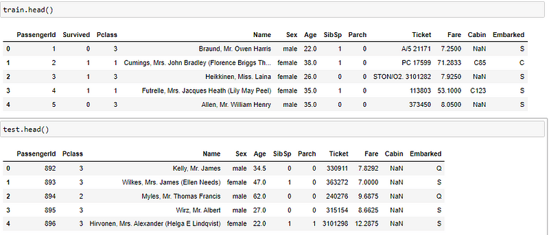
Let's display the first five rows both for trainand test .

train.head()

test.head()

---

Data Analysis and EDA.

To make things easier, let's join both the train and test dataframes to create a single dataset.

dataset=pd.concat(objs=[train, test], axis=0)
dataset=dataset.set_index("PassengerId")

The set_index method is called on dataset to set the index column as "PassengerId".

It is important to note that test dataset should not be used in this way during training, as it is meant to be used as a separate dataset to evaluate the performance of the trained model on unseen data. In practice, we should not include the test data in the training dataset, and instead only use it for testing and evaluation purposes.

Let's display the first and the last few rows of the concatenated dataset.

dataset.head()

dataset.tail()

Let's familiarize ourselves with the kind of dataset we're working with.

dataset.info()

• From the output, the dataset has 1309 entries and 11 columns - 3 columns are of type float, 3 columns are of type integer, and 5 columns are categorical columns of type object. Some of the columns have missing values. The Survived column has only 891 non-null values, which means that there are missing values in this column for the test set but keep in mind that this column was not present in the test dataset, and so we won't fill these missing values.

About the features.

The column attributes have the following meaning:

• PassengerId: a unique identifier for each passenger.
• Survived: that's the target, 0 means the passenger did not survive, while 1 means he/she survived.
• Pclass: passenger class.
• Name, Sex, Age: Self-explanatory.
• SibSp: how many siblings and spouses of the passenger aboard the Titanic.
• Parch: how many children & parents of the passenger aboard the Titanic.
• Ticket: ticket id.
• Fare: price paid (in pounds).
• Cabin: passenger's cabin number.
• Embarked: where the passenger embarked the Titanic.

Next Up: statistical summary.

dataset.describe().T

This will provide the statistical summary of the numerical columns in the dataset. The .T function transposes the table to make it more readable.

• The mean age was 29.88, and the oldest person was 80 yrs.
• The mean fare was 33.30 pounds.
• The survival rate was only 38%, quite sad 😢 .

---

Visualizations.

Let's now visualize the distribution of some key features.

#Target class
sns.set(style="white", color_codes=True)
ax=sns.catplot("Survived", data=dataset, kind="count", hue="Sex", height=5)
plt.title("Survival Distribution", weight="bold")
plt.xlabel("Survival", weight="bold", size=14)
plt.ylabel("Head Count", size=14)
ax.set_xticklabels(["Survived", "Didn't Survive"], rotation=0)
plt.show(); 

• From the generated categorical plot, we can see most men survived as compared to those who didn't. On the other hand, most women/female didn't survive as compared to those who survived. This is quite an interesting visual.

Let's continue uncovering these relationships:

sns.set(style="white", color_codes=True)
ax=sns.catplot("Survived", data=dataset, kind="count", hue="Embarked", height=5)
plt.title("Survival Distribution by boarding Place", weight="bold")
plt.xlabel("Survival", weight="bold", size=14)
plt.ylabel("Head Count", size=14)
ax.set_xticklabels(["Survived", "Didn't Survive"], rotation=0)
plt.show();

The Embarked column in this dataset indicates the port of embarkation of each passenger. The values represents:

• C: Cherbourg.
• Q: Queenstown.
• S: Southampton.

Interestingly, the survival rate of those who embarked the ship at Southampton was way more higher as compared to the rest.

Let's look at a few more:

sns.set(style="white", color_codes=True)
ax=sns.catplot("Survived", data=dataset, kind="count", hue="Pclass", height=5)
plt.title("Survival Distribution by Passenger Class", weight="bold")
plt.xlabel("Survival", weight="bold", size=14)
plt.ylabel("Head Count", size=14)
ax.set_xticklabels(["Survived", "Didn't Survive"], rotation=0)
plt.show();

• If a passenger happened to be in the 3rd class, the chances were higher that he/she would survive the incident. Paradoxically, most people who were in the first class didn't survive compared to those who survived in both 1st and 2nd classes.

To further understand the distribution of the survival outcomes, let's create a new colum age_dec that bins the Age column into decades.

dataset['age_dec']=dataset.Age.map(lambda Age:10*(Age//10))

sns.set(style="white", color_codes=True)
ax=sns.catplot("Survived", data=dataset, kind="count", hue="age_dec", height=5)
plt.title("Survival Distribution by Age Decade", weight="bold")
plt.xlabel("Survival", weight="bold", size=14)
plt.ylabel("Head Count", size=14)
ax.set_xticklabels(["Survived", "Didn't Survive"], rotation=0)
plt.show();

• The plot shows that passengers in their 20s and 30s had the highest survival rate, while those in their 1s and 60s had the lowest.

Finally, let's create a violin plot that shows the distribution of passengers by age decade and passenger class, with the hue representing the passenger's sex.

sns.violinplot(x="age_dec", y="Pclass", hue="Sex",data=dataset,
               split=True, inner='quartile',
               palette=['lightpink', 'lightblue']);

• The plot shows the distribution of passenger ages by decade and class, with the violins representing the density of passengers at different ages. The split violins allow for easy comparison of the distributions for male and female passengers within each age and class group.

---

Preprocessing.

Time to preprocess the data before feeding it into our models. But first, how many missing values do we have? and while we're at it, let's create a pandas dataframe containing the percentages of the missing values of each column.

dataset.isnull().sum()

#percentage missing
p_missing= dataset.isnull().sum()*100/len(dataset)
missing=pd.DataFrame({"columns ":dataset.columns,
                     "Missing Percentage": p_missing})
missing.reset_index(drop=True, inplace=True)
missing

• About 20% is missing both in Age and age_dec columns, the Cabin column have 77% of its values missing.

Next we need to identify which columns we will be dropping, and then split the columns into numerical and categorical columns.

col_drop=['Name','Ticket', 'Cabin']
print(f"Dataset shape before dropping: {dataset.shape}")
dataset=dataset.drop(columns=col_drop)
print(f"Dataset shape after dropping: {dataset.shape}")

#Numerical and Categorical columns
cat=[col for col in dataset.select_dtypes('object').columns]
num=[col for col in dataset.select_dtypes('int', 'float').columns if col not in ['Survived']]
print(cat)
print(num)

• The code is dropping the Name, Ticket, and Cabin columns from the dataset DataFrame, and then creating two lists cat and num.
• cat list contains the names of categorical columns in the dataset which are of object datatype while num list contains the names of numerical columns which are of int and float datatype except Survived column which is our target feature.

---

Split the dataset.

train=dataset[:891]
test=dataset[891:].drop("Survived", axis=1)

• The train dataframe contains the first 891 rows of the original dataset, which corresponds to the training data for the Titanic survival prediction problem. The test dataframe contains the remaining rows of the original dataset, which corresponds to the test data for the problem. The Survived column is dropped from the test dataframe because this is the target variable that we are trying to predict, and it is not present in the test data.

---

Transformation Pipelines.

To prepare the data for machine learning algorithms, we need to convert the data into a format that can be processed by these algorithms. One important aspect of this is to transform categorical data into numerical data, and to fill in any missing values in the data. To automate these tasks, we can create data pipelines that perform these operations for us. These pipelines will help to transform our data into a format that can be used by machine learning algorithms.

num_pipeline=Pipeline([
    ("imputer", SimpleImputer(strategy="median")),
    ("scaler", StandardScaler())
])

cat_pipeline=Pipeline([
    ("imputer", SimpleImputer(strategy="most_frequent")),
    ("encoder", OneHotEncoder())
])

full_pipeline=ColumnTransformer([
    ("cat", cat_pipeline, cat),
    ("num", num_pipeline, num)
])

• The num_pipeline first applies a SimpleImputer to fill in missing values with the median value of the column, and then standardizes the data using StandardScaler(). The cat_pipeline applies a SimpleImputer to fill in missing values with the most frequent value of the column, and then encodes the categorical variables using OneHotEncoder().

• The ColumnTransformer is then used to apply these pipelines to the respective columns in the dataset. The cat and num lists created earlier are used to specify which columns belong to each pipeline.
  

# Transform the train dataset
X_train = full_pipeline.fit_transform(train[cat+num])
X_train

• The code above applies the full_pipeline ColumnTransformer to the concatenated train dataset ( train[cat+num] ) that contains both categorical ( cat ) and numerical ( num ) columns. The output is a Numpy array that contains the transformed features.

Let's do the same for the test dataset.

X_test=full_pipeline.fit_transform(test[cat+num])
X_test

Identify the target class.

y_train=train["Survived"]

---

Classification Models.

Random Forest Classifier.

rf=RandomForestClassifier(n_estimators=200, random_state=42)
rf.fit(X_train, y_train )
y_pred=rf.predict(X_test)


scores=cross_val_score(rf, X_train, y_train, cv=20)
scores.mean()

• The above code fits the random forest classifier to the training dataset and predicts the target variable for the test dataset, later it performs 20-fold cross-validation on the training dataset by taking the random forest classifier, the predictor variables X_train, the target variable y_train, and the cv=20parameter. It returns the accuracy score for each fold. scores.mean() returns the mean accuracy score across all the folds.

Wow, the model performed amazingly - 80.01% is quite a satisfying performance considering this is our first run.

XGBoost Classifier.

Let's try out a gradient boosting classifier and see how well it performs.

model = XGBClassifier(
    n_estimators=100,
    max_depth=8,
    n_jobs=-1,
    random_state=42
)

model.fit(X_train, y_train)
y_pred=model.predict(X_test)


scores=cross_val_score(model, X_train, y_train, cv=20)
scores.mean()

• Not bad, 79% is somehow better - remember this is our first time executing these models and we're doing so without any feature engineering or hypeparameter tuning techniques.

Let's try two more extra models; a support vector one and a neural-network one to see if our performance improves.

Support Vector Machine.

svm=SVC(gamma="auto")
svm.fit(X_train, y_train)
y_pred=svm.predict(X_test)

scores=cross_val_score(svm, X_train,y_train, cv=20)
scores.mean()

• Hooray!!! our perfomace just impoved by 1%, now we're at 81% - it might seem subtle but it's quite a massive win considering the kind of task we're handling.

• This model seems promising and would be highly recommend for further development.

Multi-Layer Perceptron Classifier.

Lastly, let's create a neural network classifier to tackle the problem. MLPC classifier is a neural network algorithm mostly used for classification tasks.

nn=MLPClassifier(hidden_layer_sizes=(20,15,25))
nn.fit(X_train, y_train)
nn.predict(X_test)

scores=cross_val_score(nn, X_train, y_train, cv=15)
scores.mean()

• Not disappointing at all, the model gave us an 80.15% perfomance.

Overall, our models performed better with an average score of 80%.

PS: Your scores might be different from those herein but that's not something to worry about.

---

Fun Fact: Looking at the leaderboard for the Titanic competition on Kaggle, our scores would've been among the top 3%, ain't that not mind-blowing?.🤩😎.

But wueh, some kagglers achieved 100% score, yeah you heard me right, 100%…that's nuts, special respect to all of them. 👏

Tips to Improve performance:

• Hyperparameters tuning using GridSearch and Cross validation.
• Feature Engineering, eg, try to add some attributes such as SibSP and Parch .
• Identify parts of names that correlate well with the Survived attribute.

---

And with that, we're done with our classification model development. Let's connect on LinkedIn and Twitter.