Introduction to Neural Networks with Brain.js

What is a Neural Network

Neural Networks are incredibly useful computing structures that allow computers to process complex inputs and learn how to classify them. The functionality of a neural network comes from its structure, which is based off the patterns found in the brain.

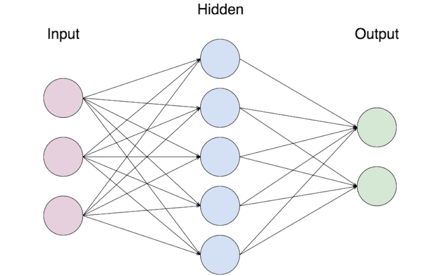
Notice that the network is divided into three distinct Layers. When a neural network is in use, it activates the layers from left to right, leading from input to output. It is also possible for there to be multiple hidden layers, but we’ll tackle that later.
Each circle in the above diagram is a Neuron. Each neuron’s job is to measure a specific variable, and the higher the layer the neuron is in, the more information that variable has. An input neuron might measure the brightness of a single pixel, neurons in the middle may describe individual elements of a picture, and an output neuron would describe the whole picture. This value is a number that fits in a specific range (like between 0 and 1), which is called the neuron’s activation. Neurons also have a second value called a bias, which changes the default value of the neuron away from 0.5.
Each neuron in a layer has a connection to every neuron in the next layer. Each of these connections has a weight, which is a value that represents how the two neurons relate to each other. A highly positive weight means that the first neuron makes the second more likely to activate, where a high negative weight means the first prevents the second from activating. A weight of 0 means the first neuron has absolutely no effect on the second.

When input data is fed into a neural network, it creates a set of activation values in the first layer. Every connection in this layer then ‘fires off’ in sequence. When a connection fires, it multiplies the activation of the left neuron by the weight of the connection, then adds that to a running total for the right neuron along with the bias. At the end of this process, every neuron in the left layer has contributed to every neuron in the right layer.
Because the resulting number can be anywhere on the number line, and activations must be between 0 and 1, we need to use a function to convert the result into the appropriate range. There are many functions that work for this purpose, such as Sigmoid. Once an activation value has been generated for every neuron in the layer, the process repeats until the output layer is reached.

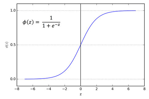
For example, in the situation below we have three nodes in the first row contributing to one node in the next. The topmost node contribute 4.0 * 0.5 = 2.0, the middle node 0.5, and the bottom node -1, which sum to 1.5. The affected node also has a bias of -2, so the total is -0.5. Plugging this value into the Sigmoid function results in a 0.378 activation value.

Okay, so we have some math that lets us shuffle some numbers around, but we can do that with any function. Why do we need to have all this business with neurons and connections and layers?

Learning

There a lot of unknowns in the neural network, every neuron in the network has a bias, and every connection between neurons has a weight. All these values can be tweaked and modified to produce neural networks that will have different behaviors. Of course, most of these possible combinations will give us entirely useless answers. How do we narrow down from the infinite possible combination to one of the few usable sets?
First, we need to define some way to tell how well any given configuration of the neural network is doing. This is done by creating a cost function, which is usually the sum of the squares of the difference between the expected and actual answers. When the cost function is high, the network is doing poorly. But when the cost function is near 0, the network is doing very well. Just knowing how well a network deals with a single sample isn’t very useful, so this is where large data sets come in. The effectiveness of a set of weights and biases is determined by running hundreds if not thousands of samples through the neural net.

If we were to plot our cost function for every possible value of the parameters, then we would have a plot similar to (but immensely more complicated than) the one above. Because this is the cost function, the lowest points on the plot represent the most accurate sets of parameters. We can therefore find the local minima of the function by using steepest descent. Steepest decent involves finding the highest slope of the nearby section of plot, and then moving away from that rise. This involves a lot of calculus I don’t have time to replicate here, and is incredibly slow.

Learning Faster with Backpropagation

Backpropagation offers a much faster way to approximate steepest descent. The key idea behind is essentially: feed a sample into the neural network, find where the answer deviates from the expected value, find the smallest tweaks you can do to get the expected answer.
This process works due to the wide branching structure of neural networks. Because neurons are fed through so many different paths, and each path has different weight associated with it, it’s possible to find values that are order of magnitude more influential on the values you care about than others. Following this process leads to a list of changes to make to existing weight and bias values. Applying just these changes will lead to overtraining your data set, so you need to get a good average before making any changes. You should shuffle your data set so that you get a random assortment of samples, generating lists of changes for each one. After averaging a few hundred of these lists together, then you can enact changes to the network. While each individual nudge resulting from this won’t be in the steepest descent, the average will eventually drag the cost function to a local minimum.

Enough with the Theory Already!

Brain is a javascript library made for easy and high-level neural networking. Brain handles almost all of the set up for you, allowing you to worry only about high level decisions.
Scaling Function: Sets the function for determining the activation value of neurons.
Number of Hidden Layers: The number of additional layers between the Input and Output layers. There is almost no reason to use more than two layers for any project. Increasing the number of layers massively increases computation time.
Iterations: The number of times the network is run through the training data before it stops.
Learning Rate: A global scalar for how much values can be tweaked. Too low, and it will take a very long time to converge to the answer. Too high, and you may miss a local minimum.

const network = new brain.NeuralNetwork({
    activation: ‘sigmoid’,  //Sets the function for activation
    hiddenLayers: [2],  //Sets the number of hidden layers
    iterations: 20000, //The number of runs before the neural net stops training
    learningRate: 0.4 //The multiplier for the backpropagation changes
}) 

The above parameters are passed into the NeuralNetwork class as an object. The network can then be trained using the .train method. This requires prepared training data. Sample data should be structured as an array of objects with input and output values. The input and output values should be an array of numbers, these correspond to the activation values of the neurons in the first and last layers of the network, respectively. Its important that the number of elements in the input and output arrays remain consistent (internally, they don’t have to be equal to each other) as this determines the number of nodes that will exist in the front and back layers of the network.

let trainingSample1 = {
    input: [ 5.3, 6 , 1 , -4 ]
    output: [ 0 , 1  ] 
}

let trainingSample2 = {
    input: [ 1 , -14 , 0.2 , 4.4 ]
    output: [ 1 , 1  ] 
} 
trainingData.push( trainingSample1 )
trainingData.push( trainingSample2 )

network.train(trainingData)

And now the network has done its level best to train itself under your chosen settings and samples. You can now use the .run command to examine the output for a given sample. And voila, your network will be able to make approximations based off of any given input. I’d say it’s like magic if you hadn’t just read 1000 words explaining how it works.

    let sample = [20, -3, -5, 13]
    let result = network.run(sample)