Basics of Object Detection (Part 1)

This article is originally from the book "Modern Computer Vision with PyTorch"

Introduction

Imagine a scenario where we are leveraging computer vision for a self-driving car. It is not only necessary to detect whether the image of a road contains the images of vehicles, a sidewalk, and pedestrians, but it is also important to identify where those objects are located. Various techniques of object detection that we will study in this article will come in handy in such a scenario.

With the rise of autonomous cars, facial detection, smart video surveillence, and people-counting solutions, fast and accurate object detection systems are in great demand. These systems include not only object classification from an image, but also location of each one of the objects by drawing appropriate bounding boxes around them. This (drawing bounding boxes and classification) makes object detection a harder task than its traditional computer vision predecessor, image classification.

To understand what the output of object detection looks like, let's go through the following diagram. In the preceding diagram, we can see that, while a typical object classification merely mentions the class of object present in the image, object localization draws a bounding box around the objects present in the image. Object detection, on the other hand, would involve drawing the bounding boxes around individual objects in the image, along with identifying the class of object within a bounding box across multiple objects present in the image.

Training a typical object detection model involves the following steps:

1. Creating ground truth data that contains labels of the bounding box and class corresponding to various objects present in the image.
2. Coming up with mechanisms that scan through the image to identify regions (region proposals) that are likely to contain objects. In this article, we will learn about leveraging region proposals generated by a method named selective search. Also, we will learn about leveraging anchor boxes to identify regions containing objects. Moreover, we will learn about leveraging positional embeddings in transformers to aid in identifying the regions containing an object.
3. Creating the target class variable by using the IoU metric.
4. Creating the target bounding box offset variable to make corrections to the location of region proposal coming in the second step.
5. Building a model that can predict the class of object along with the target bounding box offset corresponding to the region proposal.
6. Measuring the accuracy of object detection using mean Average Precision (mAP).

Creating a bounding box ground truth for training

We have learned that object detection gives us the output where a bounding box surrounds the object of interest in an image. For us to build an algorithm that detects the bounding box surrounding the object in an image, we would have to create the input-output combinations, where the input is the image and the output is the bounding boxes surrounding the objects in the given image, and the classes corresponding to the objects.

To train a model that provides the bounding box, we need the image, and also the corresponding bounding box coordinates of all the objects in an image. In this section, we will learn about one way to create the training dataset, where the image is the input and the corresponding bounding boxes and classes of objects are stored in an XML file as output. We will use the ybat tool to annotate the bounding boxes and the corresponding classes.

Let's understand about installing and using ybat to create (annotate) bounding boxes around objects in the image. Furthermore, we will also be inspecting the XML files that contain the annotated class and bounding box information.

Installing the image annotation tool

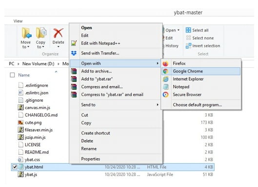
Let's start by downloading ybat-master.zip from the following github and unzip it. Post unzipping, store it in a folder of your choice. Open ybat.html using a browser of your choice and you will see an empty page. The following screenshot shows a sample of what the folders looks like and how to open the ybat.html file.

Before we start creating the ground truth corresponding to an image, let's specify all the possible classes that we want to label across images and store in the classes.txt file as follows:

Now, let's prepare the ground truth corresponding to an image. This involves drawing a bounding box around objects and assigning labels/classes to the object present in the image in the following steps:

1. Upload all the images you want to annotate
2. Upload the classes.txt file.
3. Label each image by first selecting the filename and then drawing a crosshair around each object you want to label. Before drawing a crosshair, ensure you select the correct class in the classes region.
4. Save the data dump in the desired format. Each format was independently developed by a different research team, and all are equally valid. Based on their popularity and convenience, every implementation prefers a different format.

For example, when we downlaod the PASCAL VOC format, it downloads a zip of XML files. A snapshot of the XML files after drawing the rectangular bounding box is as follows:

From the preceding screenshot, note that the bndbox field contains the coordinates of the minimum and maximum values of the x and y coordinates corresponding to the object of interest in the image. We should also be able to extract the classes corresponding to the objects in the image using the name field.

Now that we understand how to create a ground truth of objects (class labels and bounding box) present in an image, in the following sections, we will dive into the building blocks of recognizing objects in an image. First, we will talk about region proposals that help in highlighting the portions of the image that are most likely to contain an object.

Understanding region proposals

Imagine a hypothetical scenario where the image of interest contains a person and sky in the background. Furthermore, for this scenario, let's assume that there is little change in pixel intensity of the background and that there is considerable change in pixel intensity of the foreground.

Just from the preceding description itself, we can conclude that there are two primary regions here-one is of the person and the other is of the sky. Furthermore, within the region of the image of a person, the pixels corresponding to hair will have a different intensity to the pixels corresponding to the face, establishing that there can be multiple sub-regions within a region.

Region proposal is a technique that helps in identifying islands of regions where the pixels are similar to one another.

Generating a region proposal comes in handy for object detection where we have to identify the locations of objects present in the image. Furthermore, given a region proposal generates a proposal for each region, it aids in object localization where the task is to identify a bounding box that fits exactly around the object in the image. We will learn how region proposals assist in object localization and detection in a later section on Training R-CNN based custom object detectors, but let's first understand how to generate region proposals from an image.

Leveraging Selective Search to generate region proposals

Selective Search is a region proposal algorithm used for object localization where it generates proposals of regions that are likely to be ground together based on their pixel intensities. Selective Search groups pixels based on the hierarchical grouping of similar pixels, which, in turn, leverages the color, texture, size and shape compatibility of content within an image.

Initially, Selective Search over-segments an image by grouping pixels based on the preceding attributes. Next, it iterates through these over-segmented groups and groups them based on similarity. At each iteration, it combines smaller regions to form a larger region.

Let's understand the selective search process through the following example:

## dependencies 
pip install selectivesearch
pip install torch_snippets

from torch_snippets import *
import selectivesearch
from skimage.segmentation import felzenszwalb

img = read('Hemanvi.jpeg', 1)

## extract the felzenszwalb segments (which are obtained based on the color, texture, size and shape compatibility of content within an image) from the image
segments_fz = felzenszwalb(img, scale=200)

## scale represents the number of clusters that can be formed within the segments of the image. The higher the value of scale, the greater the detail of the original image that is preserved.

subplots([img, segments_fz], titles=['Original Image', 'Image post \nfelzenszwalb segmentation'], sz=10, nc=2)

The preceding code results in the following output:

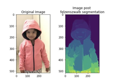
From the preceding output, note that pixels that belong to the same group have similar pixel values.

Implementing Selective Search to generate region proposals

In this section, we will define the extract_candidates function using selectivesearch so that it can be leveraged in the subsequent sections on training R-CNN and Fast R-CNN-based custom object detectors:

from torch_snippets import *
import selectivesearch 

# define the function that takes an image as the input parameter
def extract_candidates(img):
 # fetch the candidate regions within the image using the selective_search method available in the selectivesearch package
 img_lbl, regions = selectivesearch.selectivesearch(img, scale=200, min_size=100)

 # calculate the image area and initialize a list (candidates) that we will use to store the candidates that pass a defined threshold
 img_area = np.prod(img.shape[:2])
 candidates = []

 # fetch only those candidates (regions) that are over 5% of the total image area and less than or equal to 100% of the image area and return them
 for r in regions:
  if r['rect'] in candidates:
   continue
  if r['size'] < (0.05 * img_area):
   continue
  if r['size'] > (1 * img_area): 
   continue
  x, y, w, h = r['rect']
  candidates.append(list(r['rect']))
 return candidates 

img = read('Hemanvi.jpeg', 1)
candidates = extract_candidates(img)
show(img, bbs=candidates)

The preceding code generates the following output:

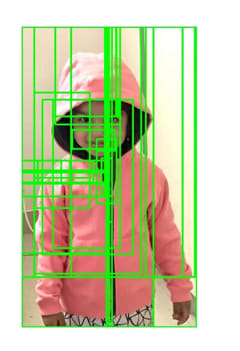
The grid in the preceding diagram represent the candidate regions (region proposals) coming from the selective_search method.

Now that we understand region proposal generation, one question remains unanswered. How do we leverage region proposals for object detection and localization?

A region proposal that has a high intersection with the location (ground truth) of an object in the image of interest is labeled as the one that contains the object, and a region proposal with a low intersection is labeled as background.

In the next section, we will learn about how to calculate the intersection of a region proposal candidate with a ground truth bounding box in our journey to understand the various techniques that form the backbone of building an object detection model.

Understanding IoU

Imagine a scenario where we came up with a prediction of a bounding box for an object. How do we measure the accuracy of our prediction? The concept Intersection over Union (IoU) comes in handy in such a scenario.

Intersection measures how overlapping the predicted and actual bounding boxes are, while Union measures the overall space possible for overlap. IoU is the ratio of the overlapping region between the two bounding boxes over the combined region of both the bounding boxes.

This can be represented in a diagram as follows:

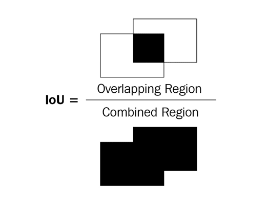
In the preceding diagram of two bounding boxes (rectangles), let's consider the left bounding box as the ground truth and the right bounding box as the prediction location of the object. IoU as a metric is the ratio of the overlapping region over the combined region between the two bounding boxes.

In the following diagram, you can observe the variation in the IoU metric as the overlap between bounding boxes varies:

From the preceding diagram, we can see that as the overlap decreases, IoU decreases and, in the final one, where there is no overlap, the IoU metric is 0.

Now that we have an intuition of measuring IoU, let's implement it in code and create a function to calculate IoU as we will leverage it in the sections of training R-CNN and training Fast R-CNN.

Let's define a function that takes two bounding boxes as input and returns IoU as the output:

# specify the get_iou function that takes boxA and boxB as inputs where boxA and boxB are two different bounding boxes
def get_iou(boxA, boxB, epsilon=1e-5):
 # we define the epsilon parameter to address the rare scenario when the union between the two boxes is 0, resulting in a division by zero error. 
 # note that in each of the bounding boxes, there will be four values corresponding to the four corners of the bounding box

 # calculate the coordinates of the intersection box
 x1 = max(boxA[0], boxB[0])
 y1 = max(boxA[1], boxB[1])
 x2 = min(boxA[2], boxB[2])
 y2 = min(boxA[3], boxB[3])

 # note that x1 is storing the maximum value of the left-most x-value between the two bounding boxes. y1 is storing the topmost y-value and x2 and y2 are storing the right-most x-value and bottom-most y-value, respectively, corresponding to the intersection part.

 # calculate the width and height corresponding to the intersection area (overlapping region):
 width = (x2 - x1)
 height = (y2 - y1)

 # calculate the area of overlap
 if (width < 0) or (height < 0):
  return 0.0
 area_overlap = width * height

 # if we specify that if the width or height corresponding to the overlapping region is less than 0, the area of intersection is 0. Otherwise, we calculate the area of overlap (intersection) similar to the way a rectangular's area is calculated. 

 # calculate the combined area corresponding to the two bounding boxes
 area_a = (boxA[2] - boxA[0]) * (boxA[3]- boxA[1])
 area_b = (boxB[2] - boxB[0]) * (boxB[3] - boxB[1])
 area_combined = area_a + area_b + area_overlap

 iou = area_overlap / (area_combined + epsilon)
 return iou