Basics of Object Detection (Part 2)

This article is originally from the book "Modern Computer Vision with PyTorch"

We will hold off on building a model until the forthcoming sections as training a model is more involved and we would also have to learn a few more components before we train it. In the next section, we will learn about non-max suppression, which helps in shortlisting from the different possible predicted bounding boxes around an object when inferring using the trained model on a new image.

Non-max suppression

Imagine a scenario where multiple region proposals are generated and significantly overlap one another. Essentially, all the predicted bounding box coordinates (offsets to region proposals) significantly overlap one another. For example, let's consider the following image, where multiple region proposals are generated for the person in the image:

In the preceding image, I ask you to identify the box among the many region proposals that we will consider as the one containing an object and the boxes that we will discard. Non-max suppression comes in handy in such a scenario. Let's unpack the term "Non-max suppression".

Non-max refers to the boxes that do not contain the highest probability of containing an object, and suppression refers to us discarding those boxes that do not contain the highest probability of containing an object. In non-max suppression, we identify the bounding box that has the highest probability and discard all the other bounding boxes that have an IoU greater than a certain threshold with the box containing the highest probability of containing an object.

In PyTorch, non-max suppression is performed using the nms function in the torchvision.ops module. The nms function takes the bounding box coordinates, the confidence of the object in the bounding box, and the threshold of IoU across bounding boxes, to identify the bounding boxes to be retained. You will be leveraging the nms function when predicting object classes and bounding boxes of objects in a new imagein both the Training R-CNN-based custom object detectors and Training Fast R-CNN-based custom object detectors sections.

Mean average precision

So far, we have looked at getting an output that comprises a bounding box around each object within the image and the class corresponding to the object within the bounding box. Now comes the next question: How do we quantify the accuracy of the predictions coming from our model?

mAP comes to the rescue in such a scenario. Before we try to understand mAP, let's first understand precision, then average precision, and finally, mAP:

• Typically we calculate precision as
  
  A true positive refers to the bounding boxes that predicted the correct class of objects and that have an IoU with the ground truth that is greater than a certain threshold. A false positive refers to the bounding boxes that predicted the class incorrectly or have an overlap that is less than the defined threshold with the ground truth. Furthermore, if there are multiple bounding boxes that are identified for the same ground truth bounding box, only one box can get into a true positive, and everything else gets into a false negative.

• Average precision is the average of precision values calculated at various IoU thresholds.

• mAP is the average of precision values calculated at various IoU threshold values across all the classes of objects present within the dataset.

So far, we have learned about preparing a training dataset for our model, performing non-max suppression on the model's predictions, and calculating its accuracies. In the following sections, we will learn about training a model (R-CNN-based and Fast R-CNN-based) to detect objects in new images.

Training R-CNN-based custom object detectors

R-CNN stands for Region-based Convolutional Neural Network. Region-based within R-CNN stands for the region proposals. Region proposals are used to identify objects within an image. Note that R-CNN assists in identifying both the object present in the image and the location of objects present in the image and the location of objects within the image.

In the following sections, we will learn about the working details of R-CNN before training it on our custom dataset.

Working details of R-CNN

Let's get an idea of R-CNN-based object detection at a high level using the following diagram:

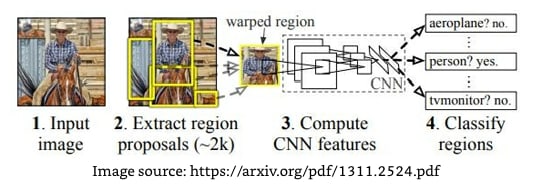
We perform the following steps when leveraging the R-CNN technique for object detection:

1. Extract region proposals from an image: ensure that we extract a high number of proposals to not miss out on any potential object within the image.
2. Resize (warp) all the extracted regions to get images of the same size.
3. Pass the resized region proposals through a network: typically we pass the resized region proposals through a pretrained model such as VGG16 or ResNet50 and extract the features in a fully connected layer.
4. Create data for model training, where the input is features extracted by passing the region proposals through a pretrained model, and the outputs are the class corresponding to each region proposal and the offset of the region proposal from the ground truth corresponding to the image. If a region proposal has an IoU greater than a certain threshold with the object, we prepare training data in such a way that the region is responsible for predicting the class of object it is overlapping with and also the offset of region proposal with the ground truth bounding box that contains the object of interest.

A sample as a result of creating a bounding box offset and a ground truth class for a region proposal is as follows:

In the preceding image, o (in red) represents the center of region proposal (dotted bounding box) and x represents the center of the ground truth bounding box (solid bounding box) corresponding to cat class. We calculate the offset between the region proposal bounding box and the ground truth bounding box as the difference between center coordinates of the two bounding boxes ($dx, dy$) and the difference between the height and width of the bounding boxes ($dw, dh$).

1. Connect two output heads, one corresponding to the class of image and the other corresponding to the offset of region proposal with the ground truth bounding box to extract the fine bounding box on the object.

2. Train the model post, writing a custom loss function that minimizes both object classification error and the bounding box offset error.

Note that the loss function that we will minimize differs from the loss function that is optimized in the original paper. We are doing this to reduce the complexity associated with building R-CNN and Fast R-CNN from scratch. Once the reader is familiar with how the model works and can build a model using the following code, we highly encourage them to implement the original paper from scratch.

In the next section, we will learn about fetching datasets and creating data for training. In the section after that, we will learn about designing the model and training it before predicting the class of objects present and their bounding boxes in a new image.

Implementing R-CNN for object detection on a custom dataset

Implementing R-CNN involves the following steps:

1. downloading the dataset
2. preparing the dataset
3. defining the region proposals extraction and IoU calculation functions
4. creating input data for the model, resizing the region proposals, passing them through a pretrained model to fetch the fully connected layer values
5. labelling each region proposal with a class or background label, defining the offset of the region proposal from the ground truth if the region proposal corresponds to an object and not background
6. defining and training the model
7. predicting on new images

Downloading the dataset

We will download the data from the Google Open Images v6 dataset. In code, we will work on only those images that are of a bus or a truck to ensure that we can train the images (as you will shortly notice the memory issues associated with using selectivesearch).

pip install -q --upgrade selectivesearch torch_snippets
mkdir -p ~/.kaggle
mv kaggle.json ~/.kaggle
ls ~/.kaggle
chmod 600 /root/.kaggle/kaggle.json
kaggle datasets download -d sixhky/open-images-bus-trucks/
unzip -qq open-images-bus-trucks.zip

By now, we have defined all the functions necessary to prepare data and initialize data loaders. In the next section, we will fetch region proposals (input regions to the model) and the ground truth of the bounding box offset along with the class of object (expected output).

Fetching region proposals and the ground truth of offset

In this section, we will learn about creating the input and output values corresponding to our model. The input constitutes the candidates that are extracted using the selectivesearch method and the output constitutes the class corresponding to candidates and the offset of the candidate with respect to the bounding box it overlaps the most with if the candidate contains an object.

R-CNN network architecture

In this section, we will learn about building a model that can predict both the class of region proposal and the offset corresponding to it in order to draw a tight bounding box around the object in the image.

1. Define a VGG backbone.
2. Fetch the features post passing the normalized crop through a pretrained model.
3. Attach a linear layer with sigmoid activation to the VGG backbone to predict the class corresponding to the region proposal.
4. Attach an additional linear layer to predict the four bounding box offsets.
5. Define the loss calculations for each of the two outputs (one to predict class and the other to predict the four bounding box offsets)
6. Train the model that predicts both the class of region proposals and the four bounding box offsets.

Predict on a new image

In this section, we will leverage the model trained so far to predict and draw bounding boxes around objects and the corresponding class of object within the predicted bounding box in new images.

1. Extract region proposals from the new image.
2. Resize and normalize each crop.
3. Feed-forward the preprocessed crops to make predictions of class and the offsets.
4. Perform non-max suppression to fetch only those boxes that have the highest confidence of containing an object.