Understanding Second-Order Optimization and K-FAC for Deep Learning
The field of deep learning has witnessed remarkable advancements, leading to the development of increasingly complex models capable of tackling intricate tasks across various domains.
These models often comprise millions, and in some cases, billions of parameters, necessitating the use of efficient optimization algorithms to facilitate effective training . The sheer scale of these models renders the training process computationally intensive, demanding substantial resources and time. Consequently, achieving faster convergence during training has become a paramount objective in both research and practical applications/
Traditional first-order optimization methods, such as Stochastic Gradient Descent (SGD) and Adam, while widely adopted due to their relative simplicity and computational efficiency per iteration, can exhibit slow convergence, particularly when navigating complex and high-dimensional loss landscapes . Their reliance solely on first-order derivative information limits their ability to efficiently explore the parameter space and can lead to prolonged training times.
First-order methods primarily utilize gradient information to update model parameters, effectively indicating the direction of the steepest descent in the loss landscape. However, they neglect the curvature of this landscape, which provides crucial information about the rate of change of the gradient . This limitation can result in slow progress, oscillations around the optimal solution, and a high sensitivity to the choice of the learning rate .
While adaptive methods like Adam adjust the learning rate based on past gradients, they may still converge rapidly to suboptimal solutions or exhibit poor generalization performance in certain scenarios . The absence of curvature awareness hinders the ability of these methods to take more direct and efficient steps towards the minimum of the loss function.
Second-order optimization methods, in contrast, leverage information about the curvature of the loss landscape, typically represented by the Hessian matrix (matrix of second-order partial derivatives) or the Fisher Information Matrix (FIM), to guide the optimization process , B_S1]. By considering the curvature, these methods can make more informed parameter updates, potentially leading to significantly faster convergence.
However, a major practical challenge associated with traditional second-order methods is the computational cost of computing and inverting the Hessian matrix, which becomes infeasible for large neural networks with millions of parameters due to its size and the complexity of inversion.
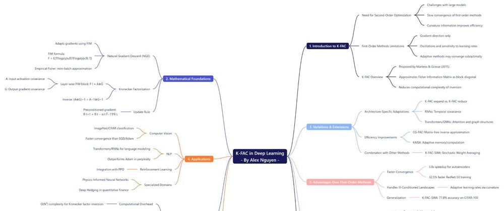
Kronecker-Factored Approximate Curvature (K-FAC) emerges as a second-order optimization method designed to address the intractability of full second-order optimization by employing Kronecker factorization to approximate the curvature.
Proposed by James Martens and Roger Grosse in 2015, K-FAC approximates the Fisher Information Matrix (FIM) as a block-diagonal matrix, where each block corresponds to the parameters of a single layer in the neural network.
Furthermore, each of these diagonal blocks is approximated by the Kronecker product of two smaller matrices . This factorization significantly reduces the computational complexity associated with inverting the curvature matrix, making second-order optimization more practical for training large-scale deep learning models.
The Mathematical Foundation of K-FAC
The mathematical underpinnings of K-FAC are rooted in the principles of Natural Gradient Descent (NGD), which utilizes the Fisher Information Matrix (FIM) to adapt the gradient based on the local curvature of the loss function , B_S1]. NGD aims to take optimization steps that are locally optimal with respect to the model's probability distribution. For a probabilistic model p(y∣x,θ), the FIM is formally defined as the expected value of the outer product of the gradient of the log-likelihood with respect to the model parameters θ , B_S1].
This matrix essentially captures how sensitive the model's output is to changes in its parameters. In practical deep learning scenarios, particularly with loss functions derived from the negative log-likelihood (common in tasks like image classification), the FIM can be interpreted as an approximation of the curvature of the loss function
For mini-batch training, an empirical estimate of the FIM, known as the Empirical Fisher, is often employed, which is computed as the mean of the outer product of the gradients over the data points within the mini-batch , B_S1]. This provides a practical way to approximate the true FIM when dealing with large datasets.
However, a significant challenge arises when considering the application of NGD to large neural networks. The FIM has dimensions N×N, where N represents the total number of parameters in the network . For modern deep learning models, this number can easily reach into the millions or even hundreds of millions, as exemplified by architectures like AlexNet or BERT-large.
Consequently, storing and inverting such an enormous matrix becomes computationally intractable due to both memory limitations and the cubic time complexity typically associated with matrix inversion algorithms . This fundamental limitation has historically hindered the direct application of NGD to training deep learning models, necessitating the development of efficient approximation techniques.
K-FAC addresses this challenge by employing Kronecker factorization as a dimensionality reduction and approximation technique for the FIM . The method begins by approximating the FIM as a block-diagonal matrix, where each block on the diagonal corresponds to the set of parameters within a single layer of the neural network .
This block-diagonal approximation effectively assumes that the parameter blocks of different layers are statistically independent, which simplifies the structure of the FIM. Crucially, each of these diagonal blocks, often referred to as Fisher blocks, is further approximated as the Kronecker product (⊗) of two smaller matrices .
For instance, in the context of a fully connected layer with a weight matrix W of size dout×din, the corresponding Fisher block Fl is approximated as the Kronecker product of the expectation of the outer product of the output gradients (E, a dout×dout matrix) and the expectation of the outer product of the input activations (E, a din×din matrix) . These smaller matrices are significantly more manageable than the full Fisher block, which would have a size of (dindout)×(dindout).
Variations and Extensions of the K-FAC Algorithm
The original K-FAC algorithm has been extended and adapted in various ways to address the specific challenges posed by different neural network architectures and to further improve its efficiency and applicability.
For neural network architectures that incorporate weight-sharing, such as Convolutional Neural Networks (CNNs), Transformers, and Graph Neural Networks (GNNs), the standard K-FAC formulation requires modifications to account for the parameter tying inherent in these designs.
To handle these cases, two primary variations of K-FAC have been proposed: K-FAC-expand and K-FAC-reduce . These variations stem from different approaches to aggregating the dimensions associated with weight-sharing when applying the K-FAC approximation
Notably, K-FAC-reduce generally exhibits faster computation and lower memory complexity compared to K-FAC-expand, making it a more appealing choice for certain architectures and resource-constrained scenarios . Importantly, both K-FAC-expand and K-FAC-reduce have been shown to be exact for deep linear networks with weight-sharing under specific conditions, providing a theoretical basis for their effectiveness in more complex, non-linear settings .
In an effort to further reduce the computational and memory demands of K-FAC, iterative methods like CG-FAC have been developed . CG-FAC is a novel iterative algorithm that employs the Conjugate Gradient (CG) method to approximate the natural gradient, thereby avoiding the explicit computation and inversion of the Kronecker factors .
As a matrix-free approach, CG-FAC does not require the explicit generation or storage of the potentially large Fisher Information Matrix or its constituent Kronecker factors, which can be particularly advantageous when training very large models where memory resources are limited . Consequently, CG-FAC demonstrates lower time and memory complexity compared to the standard K-FAC algorithm, enhancing its scalability for training large-scale deep learning models .
Beyond these general extensions, significant research has focused on adapting K-FAC for specific neural network architectures. For Recurrent Neural Networks (RNNs), K-FAC has been modified to account for the temporal dependencies inherent in sequential data . These adaptations often involve modeling the covariance structure between gradient contributions at different time steps.
Similarly, extensions have been proposed for Convolutional Neural Networks (CNNs) to handle the unique structure and weight-sharing characteristics of convolutional layers . Recent efforts have also concentrated on applying K-FAC to Transformer architectures, which have become prevalent in natural language processing and are increasingly used in computer vision.
These adaptations often need to address the intricacies of the attention mechanism. Furthermore, there is growing interest in adapting K-FAC for Graph Neural Networks (GNNs) to leverage curvature information when learning from graph-structured data . These architecture-specific modifications often involve tailored approximations to the FIM that exploit the structural properties and weight-sharing mechanisms of each network type.
In addition to these variations, K-FAC has been effectively combined with other optimization strategies to further enhance its performance. One notable example is the integration of K-FAC with Stochastic Weight Averaging (SWA), which has been shown to improve the generalization performance of deep learning models trained with second-order optimization.
Empirical evidence suggests that the SWA variant of K-FAC can outperform different variants of SGD and Adam in terms of test accuracy . The underlying principle is that SWA helps K-FAC converge to a more robust region in the weight space, leading to better generalization.
Applications of K-FAC in Deep Learning
K-FAC has found applications across a diverse range of deep learning tasks and domains, demonstrating its versatility and potential to improve training efficiency and model performance.
In the realm of computer vision, K-FAC has been extensively applied to image classification tasks on standard benchmark datasets like ImageNet and CIFAR . It has also been utilized in object detection models, including architectures such as Mask R-CNN . In these applications, K-FAC has often shown the ability to achieve comparable or even better performance than first-order methods, frequently requiring fewer training iterations to reach the desired accuracy .
K-FAC has also been successfully applied to language modeling and natural language processing tasks, particularly with Recurrent Neural Networks (RNNs) and increasingly with Transformer architectures .
Studies have indicated that K-FAC can outperform first-order optimizers like SGD and Adam in these domains . Recent research is actively exploring the use of K-FAC for training large language models (LLMs), where efficient optimization is crucial due to the scale of these models .
In the field of reinforcement learning, K-FAC has been integrated with algorithms like Proximal Policy Optimization (PPO) to improve the training of agents . The use of K-FAC in this context can lead to more stable and efficient learning processes .
Beyond standard supervised and reinforcement learning, K-FAC has also found applications in Bayesian deep learning and variational inference. It can be used as a Hessian approximation in Laplace approximations for Bayesian neural networks and is also employed in natural gradient variational inference to facilitate efficient updates of the approximate posterior distribution .
Furthermore, recent research has explored the use of K-FAC in specialized domains. For instance, it has been applied to training Physics-Informed Neural Networks (PINNs) for solving partial differential equations (PDEs), showing promising results . K-FAC has also been used in quantitative finance for Deep Hedging, demonstrating improvements in convergence and hedging efficacy compared to first-order methods , B_S6].
Advantages of K-FAC over First-Order Optimization Methods
One of the primary advantages of K-FAC is its potential to achieve faster convergence rates compared to first-order methods like SGD and Adam, often requiring fewer iterations to reach a desired level of performance .
This can translate to a substantial reduction in the overall wall-clock time needed for training, particularly for large and complex models . For example, when training an 8-layer autoencoder, K-FAC has been shown to converge to the same loss as SGD with Momentum in significantly less time and with fewer updates .
Furthermore, second-order methods like K-FAC are generally more effective at handling ill-conditioned loss landscapes compared to first-order methods . By utilizing curvature information, K-FAC can adapt the effective learning rate for each parameter individually, allowing for more efficient progress even when the loss landscape has varying sensitivities in different directions .
While some studies suggest that SGD might lead to better generalization, combining K-FAC with techniques like Stochastic Weight Averaging (SWA) has shown promise in bridging this gap and even outperforming SGD and Adam in terms of test accuracy in certain cases . The ability of K-FAC to explore the weight space differently might contribute to improved generalization when used in conjunction with appropriate strategies.
The following table summarizes some empirical performance comparisons of K-FAC with SGD and Adam:
| Task/Architecture | Optimizer | Performance Metric | Value | Snippet(s) |
| 8-layer Autoencoder | K-FAC | Time to convergence | 3.8x faster than SGD | |
| 8-layer Autoencoder | K-FAC | Updates to convergence | 14.7x fewer than SGD | |
| CIFAR-100 (VGG16) | K-FAC-SWA | Top-1 Accuracy | 75.10% | |
| CIFAR-100 (VGG16) | SGD-SWA | Top-1 Accuracy | 74.90% | |
| CIFAR-100 (VGG16) | Adam-SWA | Top-1 Accuracy | 71.70% | |
| CIFAR-100 (PreResNet110) | K-FAC-SWA | Top-1 Accuracy | 77.80% | |
| CIFAR-100 (PreResNet110) | SGD-SWA | Top-1 Accuracy | 77.50% | |
| CIFAR-100 (PreResNet110) | Adam-SWA | Top-1 Accuracy | 75.40% | |
| ResNet-50 (ImageNet) | KFAC | Convergence Speed | Faster per iteration than SGD/Adam | |
| ResNet-50 (ImageNet) | mL-BFGS | Convergence Speed | Much faster per iteration than SGD/Adam | |
| ResNet-50 (ImageNet) | KFAC | Wall-clock time | Significantly diminished by compute costs compared to SGD/Adam | |
| ResNet-32 (CIFAR-10) | K-FAC | Iterations to Convergence | Fewer than SGD | |
| ResNet-50, Mask R-CNN, U-Net, BERT | KAISA (K-FAC) | Convergence Speed | 18.1–36.3% faster than original optimizers | |
| ResNet-50 (KAISA) | KAISA (K-FAC) | Convergence Speed (fixed memory) | 32.5% faster than momentum SGD | |
| BERT-Large (KAISA) | KAISA (K-FAC) | Convergence Speed (fixed memory) | 41.6% faster than Fused LAMB | |
| RNN (PTB, DNC) | K-FAC (proposed) | Performance | Stronger than SGD, Adam, Adam+LN | |
| Deep Hedging (LSTM) | K-FAC | Transaction Costs Reduction | 78.3% compared to Adam | , B_S6 |
| Deep Hedging (LSTM) | K-FAC | P&L Variance Reduction | 34.4% compared to Adam | , B_S6 |
| Deep Hedging (LSTM) | K-FAC | Sharpe Ratio | 0.0401 (vs -0.0025 for Adam) | , B_S6 |
Limitations and Practical Challenges of Using K-FAC
Despite its advantages, K-FAC also presents several limitations and practical challenges that need to be considered.
The computation and inversion of the Kronecker factors introduce a computational overhead, with a complexity that can be significant, potentially reaching O(N3) in some cases , B_S2]. This overhead can make each iteration of K-FAC slower than that of first-order methods . The frequency of updating the FIM approximation is a critical hyperparameter that requires careful tuning to balance computational cost and convergence benefits .
K-FAC also typically requires storing per-layer activations and gradients, leading to a larger memory footprint compared to SGD , B_S2]. For very large models, these increased memory demands can pose a significant challenge . Variations like CG-FAC aim to mitigate this by reducing memory usage .
Implementing K-FAC often involves modifying the model code to register layer information , B_S4], which can add complexity to existing deep learning workflows . The need for architecture-specific adaptations further contributes to this complexity .
The performance of K-FAC can be sensitive to hyperparameter tuning, particularly the damping factor, which is crucial for numerical stability . Finding the optimal hyperparameters often requires extensive experimentation .
Finally, while K-FAC has shown promise across various architectures, its effectiveness can vary depending on the specific model and task . It might not always outperform well-tuned first-order methods , and its benefits might be more pronounced in certain scenarios .
Implementation Details in Popular Deep Learning Frameworks
TensorFlow provides a tensorflow.contrib.kfac module (though its status might vary with TensorFlow versions) for implementing K-FAC , B_S4]. Using it typically involves registering layer inputs, weights, and pre-activations with a LayerCollection , B_S4]. The optimization is then performed using the KfacOptimizer , B_S4], and the preconditioner needs periodic updates during training , B_S4].
In PyTorch, while there isn't an official built-in K-FAC implementation, several third-party implementations are available , B_S5]. These implementations might have limitations such as supporting only single-GPU training or specific layer types , B_S5], and users might need to adapt the code for multi-GPU setups or custom layers , B_S5]. Performance comparisons between TensorFlow and PyTorch implementations have been discussed within the community .
Recent Research and Advancements in K-FAC
Recent research continues to focus on improving the scalability and efficiency of K-FAC. Frameworks like KAISA have been developed to adapt memory, communication, and computation for large models . Iterative methods like CG-FAC aim to reduce computational and memory overhead . Exploration of layer-wise distribution strategies and inverse-free gradient evaluation is also ongoing .
New theoretical insights include extensions like K-FAC-expand and K-FAC-reduce for handling linear weight-sharing layers , and novel algorithms like K-FOC for optimal FIM computations . Research also explores connections between K-FAC heuristics and other optimization methods .
Applications of K-FAC are expanding to novel deep learning architectures and tasks, including Physics-Informed Neural Networks (PINNs) , Deep Hedging in quantitative finance , B_S6], and training Transformers and Graph Neural Networks (GNNs) .
Assessing the Role and Future of K-FAC in Deep Learning Optimization
Kronecker-Factored Approximate Curvature (K-FAC) represents a significant advancement in the realm of second-order optimization for deep learning. Its core strength lies in providing a computationally tractable approximation of the Fisher Information Matrix, enabling faster convergence in many scenarios compared to traditional first-order methods like SGD and Adam.
The ability of K-FAC to handle ill-conditioned loss landscapes more effectively and its potential for improved generalization, especially when combined with techniques like Stochastic Weight Averaging, make it a valuable tool for training complex neural networks.
However, the use of K-FAC is not without its challenges. The computational overhead associated with Kronecker factor computation and inversion, coupled with increased memory requirements and the complexity of implementation, can pose practical limitations. Furthermore, the performance of K-FAC can be sensitive to hyperparameter tuning and might vary across different network architectures and problem domains.
Despite these limitations, ongoing research and development are actively addressing these challenges. Efforts to improve the scalability and efficiency of K-FAC, along with the development of new theoretical insights and extensions for modern architectures, indicate a promising future for this optimization technique.
Its successful application in diverse domains, ranging from computer vision and natural language processing to reinforcement learning, Bayesian deep learning, and even specialized areas like physics-informed neural networks and quantitative finance, underscores its versatility and potential impact.
In conclusion, K-FAC stands as a powerful alternative to first-order optimization methods, particularly in scenarios where faster convergence is desired or when dealing with complex loss landscapes. While practical considerations regarding computational cost and implementation complexity remain important, continued research and the development of more efficient and user-friendly implementations are likely to further solidify the role of K-FAC in the deep learning optimization landscape.
Hi, I'm Alex Nguyen. With 10 years of experience in the financial industry, I've had the opportunity to work with a leading Vietnamese securities firm and a global CFD brokerage. I specialize in Stocks, Forex, and CFDs - focusing on algorithmic and automated trading.
I develop Expert Advisor bots on MetaTrader using MQL5, and my expertise in JavaScript and Python enables me to build advanced financial applications. Passionate about fintech, I integrate AI, deep learning, and n8n into trading strategies, merging traditional finance with modern technology.

Top comments (0)