
We have seen basics of Machine Learning, Classification and Regression. In this article, we will dive a little deeper and work on how we can do audio classification. We will train Convolution Neural Network, Multi Layer Perceptron and SVM for this task. The same code can be easily extended to train other classification models as well. I strongly recommend you to go through previous articles on basics of Classification if you haven't already done.
The main question here is to how we can handle audio files and convert it into a form which we can feed into our neural networks.
It will take less than an hour to setup and get your first working audio classifier! So let's get started! 😉
Dependencies
We will be using python. Before we can begin coding, we need to have below modules. This can be easily downloaded using pip.
- keras
- librosa
- sounddevice
- SoundFile
- scikit-learn
- matplotlib
Dataset
We are going to use ESC-10 dataset for sound classification. It is a labeled set of 400 environmental recordings (10 classes, 40 clips per class, 5 seconds per clip). It is a subset of the larger ESC-50 dataset
Each class contains 40 .ogg files. The ESC-10 and ESC-50 datasets have been prearranged into 5 uniformly sized folds so that clips extracted from the same original source recording are always contained in a single fold.
Visualize Dataset
Before we can extract features and train our model, we need to visualize waveform for the different classes present in our dataset.
import matplotlib.pyplot as plt
import numpy as np
import wave
import soundfile as sf
The below function visualize_wav() takes an ogg file, reads it using soundfile module and returns the data and sample rate. We can use sf.wav() function to write wav file for the corresponding ogg file. Using matplotlib, we are plotting signal wave across time and generating the plot.
def visualize_wav(oggfile):

    data, samplerate = sf.read(oggfile)

    if not os.path.exists('sample_wav'):
        os.mkdir('sample_wav')

    sf.write('sample_wav/new_file.wav', data, samplerate)
    spf = wave.open('sample_wav/new_file_Fire.wav')
    signal = spf.readframes(-1)
    signal = np.fromstring(signal,'Int16')

    if spf.getnchannels() == 2:
        print('just mono files. not stereo')
        sys.exit(0)

    # plotting x axis in seconds. create time vector spaced linearly with size of audio file. divide size of signal by frame rate to get stop limit
    Time = np.linspace(0,len(signal)/samplerate, num = len(signal))
    plt.figure(1)
    plt.title('Signal Wave Vs Time(in sec)')
    plt.plot(Time, signal)
    plt.savefig('sample_wav/sample_waveplot_Fire.png', bbox_inches='tight')
    plt.show()
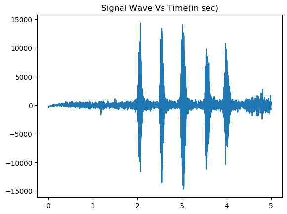
You can run the same code to generate wave plot for different classes and visualize the difference.
Feature Extraction
For each audio file in the dataset, we will extract MFCC (mel-frequency cepstrum - we will have an image representation for each audio sample) along with it’s classification label. For this we will use Librosa’s mfcc() function which generates an MFCC from time series audio data.
get_features() takes an .ogg file and extracts mfcc using Librosa library.
def get_features(file_name):

    if file_name:
        X, sample_rate = sf.read(file_name, dtype='float32')

    # mfcc (mel-frequency cepstrum)
    mfccs = librosa.feature.mfcc(y=X, sr=sample_rate, n_mfcc=40)
    mfccs_scaled = np.mean(mfccs.T,axis=0)
    return mfccs_scaled
The dataset is downloaded inside a folder "dataset". We will iterate through the subdirectories (each class) and extract features from their ogg files. Finally we will create a dataframe with mfcc feature and corresponding class label.
def extract_features():

    # path to dataset containing 10 subdirectories of .ogg files
    sub_dirs = os.listdir('dataset')
    sub_dirs.sort()
    features_list = []
    for label, sub_dir in enumerate(sub_dirs):
        for file_name in glob.glob(os.path.join('dataset',sub_dir,"*.ogg")):
            print("Extracting file ", file_name)
            try:
                mfccs = get_features(file_name)
            except Exception as e:
                print("Extraction error")
                continue
            features_list.append([mfccs,label])

    features_df = pd.DataFrame(features_list,columns = ['feature','class_label'])
    print(features_df.head())
    return features_df
Train model
Once we have extracted features, we need to convert them into numpy array so that they can be feeded into neural network.
def get_numpy_array(features_df):

    X = np.array(features_df.feature.tolist())
    y = np.array(features_df.class_label.tolist())
    # encode classification labels
    le = LabelEncoder()
    # one hot encoded labels
    yy = to_categorical(le.fit_transform(y))
    return X,yy,le
X and yy are splitted into train and test data in ratio 80-20.
def get_train_test(X,y):

    X_train, X_test, y_train, y_test = train_test_split(X,y,test_size = 0.2, random_state = 42)
    return  X_train, X_test, y_train, y_test
Now we will define our model architecture. We will use Keras for creating our Multi Layer Perceptron network.
def create_mlp(num_labels):

    model = Sequential()
    model.add(Dense(256,input_shape = (40,)))
    model.add(Activation('relu'))
    model.add(Dropout(0.5))

    model.add(Dense(256,input_shape = (40,)))
    model.add(Activation('relu'))
    model.add(Dropout(0.5))

    model.add(Dense(num_labels))
    model.add(Activation('softmax'))
    return model
Once the model is defined, we need to compile it by defining loss, metrics and optimizer. The model is then fitted to training data X_train and y_train. Our model is trained for 100 epochs with a batch size of 32. The trained model is finally saved as .hd5 file in the disk. This model can be loaded later for prediction.
def train(model,X_train, X_test, y_train, y_test,model_file):

    # compile the model
    model.compile(loss = 'categorical_crossentropy',metrics=['accuracy'],optimizer='adam')

    print(model.summary())

    print("training for 100 epochs with batch size 32")

    model.fit(X_train,y_train,batch_size= 32, epochs = 100, validation_data=(X_test,y_test))

    # save model to disk
    print("Saving model to disk")
    model.save(model_file)
This is it! We have trained our Environmental Sound Classifier!! 😃
Compute Accuracy
Now obviously we want to check how well our model is performing 😛
def compute(X_test,y_test,model_file):

    # load model from disk
    loaded_model = load_model(model_file)
    score = loaded_model.evaluate(X_test,y_test)
    return score[0],score[1]*100
Test loss 1.5628961682319642
Test accuracy 78.7
Make Predictions
We can also predict the class label for any input file we provide using below code -
def predict(filename,le,model_file):

    model = load_model(model_file)
    prediction_feature = extract_features.get_features(filename)
    if model_file == "trained_mlp.h5":
        prediction_feature = np.array([prediction_feature])
    elif model_file == "trained_cnn.h5":
        prediction_feature = np.expand_dims(np.array([prediction_feature]),axis=2)

    predicted_vector = model.predict_classes(prediction_feature)
    predicted_class = le.inverse_transform(predicted_vector)
    print("Predicted class",predicted_class[0])
    predicted_proba_vector = model.predict_proba([prediction_feature])

    predicted_proba = predicted_proba_vector[0]
    for i in range(len(predicted_proba)):
        category = le.inverse_transform(np.array([i]))
        print(category[0], "\t\t : ", format(predicted_proba[i], '.32f') )
This function will load our pre-trained model, extract mfcc from the input ogg file you have provided and output range of probabilities for each class. The one with maximum probability is our desired class! 😃
For a sample ogg file of dog class, following were the probability predictions -
Predicted class 0
0                :  0.96639919281005859375000000000000
1                :  0.00000196780410988139919936656952
2                :  0.00000063572736053174594417214394
3                :  0.00000597824555370607413351535797
4                :  0.02464177832007408142089843750000
5                :  0.00003698830187204293906688690186
6                :  0.00031352625228464603424072265625
7                :  0.00013375715934671461582183837891
8                :  0.00846461206674575805664062500000
9                :  0.00000165236258453660411760210991
The class predicted is 0 which was the class label for Dog.
Conclusion
Working on audio files is not that tough as it sounded in the first place. Audio files can easily be represented in form of time series data. We have predefined libraries in python which makes our task more simpler.
You can also check the entire code for this in my Github repo. Here I have trained SVM, MLP and CNN for the same dataset and code is arranged in proper files which makes it easy to understand.
https://github.com/apoorva-dave/Environmental-Sound-Classification
Though I have trained 3 different models for this, there was very little variance in accuracy among them. Do leave comments if you find any way to improve this score.
If you liked the article do show some ❤ Stay tuned for more! Till then happy learning 😸

Oldest comments (4)
Just my two cents, but maybe you'd get better results using more features, as RMS power, attack/release time...
i want some help , can i get your email or other contact
I am a big fan of your tutorials. I learnt concepts of machine learning within small span of time.
Thank you so much 😊😊