Linear Regression predicts a value based on an independent variable. It assumes that there is a linear relationship between input (X) and output (Y). Linear Regression is a supervised machine learning algorithm and it works best with continuous variables. Supervised machine learning means that it has labeled training data .
In linear regression, there are two types of variables:
- Dependent or outcome variable which is the variable we want to predict.
- Independent or predictor variable which is the variable used for the prediction.
Applications of linear regression models
- It establishes the relationship between values. For instance, an Ice cream vendor may want to know the relationship between the temperature of the day and the revenue collected. They can find out that on hot days, the sales are higher than on cold days.
- It's used in predictive analytics or forecasting. An insurance company can detect fraudulent claims based on previous data.
- It's used to optimize business processes by analyzing factors affecting sales. This can be factors like pricing and marketing strategies.
- It's used to support business decisions by evaluating trends.
There are two basic types of linear regression:
- Simple linear regression - It has one independent variable.
- Multiple linear regression - It has two or more independent variables.
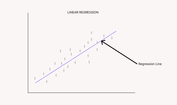
The regression line is a line that minimizes the error between predicted values and actual values.
The regression equation is represented as:
Y = mX + c
Where:
Y : is the dependent variable
m : is the scope
X : is the independent variable
c : is the intercept
m and c are derived by minimizing the sum of the squared difference of distance between the data points and the regression line. The goal of the equation is to reduce the difference between ya (actual) and yp (predicted).
How to update m and c to get the line of best fit
- Ordinary Least Squares
Ordinary Least Squares or Least square method treats the data as a matrix. It uses linear algebra to estimate the optimal values for the m and c coefficients. To use this method, all the data must be available and must fit in memory.
- Gradient descent
To optimize the values of the coefficients, gradient descent minimizes the error of your model on your training data. It starts with random coefficients and then calculates the sum of errors for each input and output value. Using the learning rate, the coefficients are updated in the direction of minimizing the error.
Learning rate is a parameter that determines the size of the improvement step to take with each iteration. This method is useful when you have a large data set that doesn’t fit in memory.
- Cost function
This is also known as Root Mean Square Error. It is the square of the difference between ya (actual) and yp (predicted) divided by N (Number of observations).
-
Regularization
Regularization methods aim to minimize squared error using Ordinary Least Squares and to reduce the complexity of the model. There are two popular examples :- Lasso Regression or L1. The Ordinary Least Square is modified to minimize the absolute sum of coefficients.
- Ridge Regression or L2. The Ordinary Least Square is modified to minimize the squared absolute sum of coefficients.
Assumptions made when building a linear regression model.
To ensure that a linear regression model achieves its intended purpose and high accuracy, it makes some assumptions about the data. Here are some of the assumptions:
Linear assumption
The model assumes that the Dependent variable and Independent variable must have a linear relationship. This relationship is best shown using a scatter plot between the dependent and independent variables.Noiseless data
Noise in data can be outliers. We use Box plots or outlier detection algorithms to detect outliers. You can either drop an outlier or replace it with the median or mean. It is most important to remove outliers from the output variable.No multicollinearity
Multicollinearity happens when you can derive an independent variable from other independent variables. Use a heatmap to detect correlating variables if the data set is small. Use VIF (Variance Inflation Factor) if the dataset is large.
If VIF=1, Very Less Multicollinearity
VIF<5, Moderate Multicollinearity
VIF>5, Extreme Multicollinearity
Removing the column with the highest VIF fixes multicollinearity.
Re-scaled inputs
Re-scale the data during the data preparation stage by standardization or normalization. This ensures that the model makes more reliable predictions.Gaussian distribution
Gaussian distribution is another term for normal distribution. Ensure that all input and output variables have gaussian distribution. If a variable is not, you can use Log Transformation or BoxCox to fix this.No autocorrelation in residuals
A residual is a deviation from the fitted line to the observed values. Use the Durbin-Watson Test to check for autocorrelation.
DW = 2 shows no autocorrelation
0 < DW < 2 shows positive autocorrelation
2 < DW < 4 shows negative autocorrelation
Statsmodels’ linear regression summary gives us the Durbin-Watson value among other useful insights.
Conclusion
This article was a brief explanation of what Linear regression is. We have also covered its applications and the different methods we can use to improve the performance of linear regression models. I hope it was helpful. Comment your thoughts and questions below.

Top comments (2)
Good explanation , also remember to add explanation about univariate and multivariate .
I like your article it has also the cost function which I don't find in many articles it helps to understand it well.
I also write a blog on linear regression anyone can also visit it and let me know your thoughts: - linear regression