Get Started With Pandas In 5 mins
A tutorial walkthrough of Python Pandas Library
For those of you who are getting started with Machine learning, just like me, would have come across Pandas, the data analytics library. In the rush to understand the gimmicks of ML, we often fail to notice the importance of this library. But soon you will hit a roadblock where you would need to play with your data, clean and perform data transformations before feeding it into your ML model.
Why do we need this blog when there are already a lot of documentation and tutorials? Pandas, unlike most python libraries, has a steep learning curve. The reason is that you need to understand your data well in order to apply the functions appropriately. Learning Pandas syntactically is not going to get you anywhere. Another problem with Pandas is that there is that there is more than one way to do things. Also, when I started with Pandas it’s extensive and elaborate documentation was overwhelming. I checked out the cheatsheets and that scared me even more.
In this blog, I am going to take you through Pandas functionalities by cracking specific use cases that you would need to achieve with a given data.
Setup and Installation
Before we move on with the code for understanding the features of Pandas, let’s get Pandas installed in your system. I advise you to create a virtual environment and install Pandas inside the virtualenv.
Create virtualenv
virtualenv -p python3 venv
source venv/bin/activate
Install Pandas
pip install pandas
Jupyter Notebook
If you are learning Pandas, I would advise you to dive in and use a jupyter notebook for the same. The visualization of data in jupyter notebooks makes it easier to understand what is going on at each step.
pip install jupyter
jupyter notebook
Jupyter by default runs in your system-wide installation of python. In order to run it in your virtualenv follow the link and create a user level kernel https://anbasile.github.io/programming/2017/06/25/jupyter-venv/
Sample Data
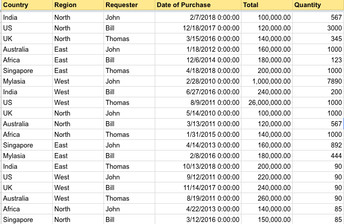
I created a simple purchase order data. It comprises of sales data of each salesperson of a company over countries and their branches at different regions in each country. Here is a link to the spreadsheet for you to download.
Load data into Pandas
With Pandas, we can load data from different sources. Few of them are loading from CSV or a remote URL or from a database. The loaded data is stored in a Pandas data structure called DataFrame. DataFrame’s are usually refered by the variable name df . So, anytime you see df from here on you should be associating it with Dataframe.
From CSV File
import pandas
df = pandas.read\_csv("path\_to\_csv")
From Remote URL
You can pass a remote URL to the CSV file in read_csv.
import pandas
df = pandas.read\_csv("remote/url/path/pointing/to/csv")
From DB
In order to read from Database, read the data from DB into a python list and use DataFrame() to create one
db = # Create DB connection object
cur = db.cursor()
cur.execute("SELECT \* FROM \<TABLE\>")
**df = pd.DataFrame(cur.fetchall())**
Each of the above snippets reads data from a source and loads it into Pandas’ internal data structure called DataFrame
Understanding Data
Now that we have the Dataframe ready let’s go through it and understand what’s inside it
**# 1. shows you a gist of the data**
df.head()

**# 2. Some statistical information about your data**
df.describe()

**# 3. List of columns headers**
df.columns.values

Pick & Choose your Data
Now that we have loaded our data into a DataFrame and understood its structure, let’s pick and choose and perform visualizations on the data. When it comes to selecting your data, you can do it with both Indexesor based on certain conditions. In this section, let’s go through each one of these methods.
Indexes
Indexes are labels used to refer to your data. These labels are usually your column headers. For eg., Country, Region, Quantity Etc.,
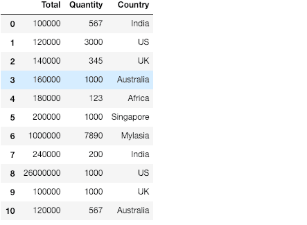
Selecting Columns
**# 1. Create a list of columns to be selected**
columns\_to\_be\_selected = ["Total", "Quantity", "Country"]

**# 2. Use it as an index to the DataFrame**
df[columns\_to\_be\_selected]

**# 3. Using loc method**
df.loc[columns\_to\_be\_selected]
Selecting Rows
Unlike the columns, our current DataFrame does not have a label which we can use to refer the row data. But like arrays, DataFrame provides numerical indexing(0, 1, 2…) by default.
**# 1. using numerical indexes - iloc**
df.iloc[0:3, :]
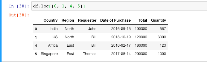
**# 2. using labels as index - loc**
row\_index\_to\_select = [0, 1, 4, 5]
df.loc[row\_index\_to\_select]
Filtering Rows
Now, in a real-time scenario, you would most probably not want to select rows based on an index. An actual real-life requirement would be to filter out the rows that satisfy a certain condition. With respect to our dataset, we can filter by any of the following conditions
**1. Total sales \> 200000**
df[df["Total"] \> 200000]

**2. Total sales \> 200000 and in UK**
df[(df["Total"] \> 200000) & (df["Country"] == "UK")]
Playing With Dates
Most of the times when dealing with date fields we don’t use them as it is. Pandas make it really easy for you to project Date/Month/Year from it and perform operations on top of it
In our sample dataset, the Date_of_purchase is of type string, hence the first step would be to convert them to the DateTime type.
\>\>\> type(df['Date of Purchase'].iloc[0])
**str**
Converting Column to DateTime Object
\>\>\> df['Date of Purchase'] = pd.to\_datetime(df['Date of Purchase'])
\>\>\> type(df['Date of Purchase'].iloc[0])
**pandas.\_libs.tslibs.timestamps.Timestamp**
Extracting Date, Month & Year
df['Date of Purchase'].dt.date **# 11-09-2018**
df['Date of Purchase'].dt.day **# 11**
df['Date of Purchase'].dt.month **# 09**
df['Date of Purchase'].dt.year **# 2018**
Grouping
Statistical operations
You can perform statistical operations such as min, max, mean etc., over one or more columns of a Dataframe.
df["Total"].sum()
df[["Total", "Quantity"]].mean()
df[["Total", "Quantity"]].min()
df[["Total", "Quantity"]].max()
df[["Total", "Quantity"]].median()
df[["Total", "Quantity"]].mode()
Now in a real-world application, the raw use of these statistical functions are rare, often you might want to group data based on specific parameters and derive a gist of the data.
Let’s look at an example where we look at the country-wise, country & Region-wise sales.
**# 1. Country wise sales and Quantity**
df.groupby("Country").sum()

**# 2. Quantity of sales over each country & Region**
df.groupby(["Country", "Region"])["Quantity"].sum()

**# 3. More than one aggregation**
df.groupby(["Country", "Region"]).agg(
 {'Total':['sum', 'max'],
 'Quantity':'mean'})

Pivot Table
Pivot Table is an advanced version of groupby, where you can stack dimensions over both rows and columns. i.e., as the data grows the groupby above is going to grow in length and will become hard to derive insights, hence a well-defined way to look at it would be Pivot tables
import numpy as np
df.pivot\_table(index=["Country"],
 columns=["Region"],
 values=["Quantity"],
 aggfunc=[np.sum])

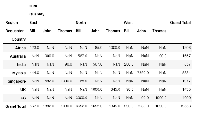
Another advantage of the Pivot Table is that you can add as many dimensions and functions you want. It also calculates a grand total value for you
import numpy as np
df.pivot\_table(index=["Country"],
 columns=["Region","Requester"],
 values=["Quantity"],
 aggfunc=[np.sum],
 **margins=True,
 margins\_name="Grand Total"** )
Okay, that was a lot of information in 5 minutes. Take some time in trying out the above exercises. In the next blog, I will walk you through some more deeper concepts and magical visualizations that you can create with Pandas.
Every time you start learning Pandas, there is a good chance that you may get lost in the Pandas jargons like index, functions, numpy etc., But don’t let that get to you. What you really have to understand is that Pandas is a tool to visualize and get a deeper understanding of your data.
With that mindset take a sample dataset from your spreadsheet and try deriving some insights out of it. Share what you learn. Here is the link to my jupyter notebook for you to get started.
Did the blog nudge a bit to give Pandas another chance?
Hold the “claps” icon and give a shout out to me on twitter. Follow to stay tuned on future blogs

Top comments (0)