How to train YOLOv7 object detection on a custom dataset using Ikomia API
With the Ikomia API, we can train a custom YOLOv7 model with just a few lines of code. To get started, you need to install the API in a virtual environment.
How to install a virtual environment
pip install ikomia
In this tutorial, we will use the aerial airport dataset from Roboflow. You can download this dataset by following this link: Dataset Download Link.
Run the train YOLOv7 algorithm with a few lines of code using Ikomia API
You can also charge directly the open-source notebook we have prepared.
from ikomia.dataprocess.workflow import Workflow
from ikomia.utils import ik

# Initialize the workflow
wf = Workflow()

# Add the dataset loader to load your custom data and annotations
dataset = wf.add_task(ik.dataset_yolo(
    dataset_folder="path/to/aerial/dataset/train",
    class_file="path/to/aerial/dataset/train/_darknet.labels")
)

# Add the Yolov7 training algorithm
yolo = wf.add_task(ik.train_yolo_v7(
    batch_size="4",
    epochs="10",
    output_folder="path/to/output/folder"),
    auto_connect=True
)

# Launch your training on your data
wf.run()
The training process for 10 epochs was completed in approximately 14 minutes using an NVIDIA GeForce RTX 3060 Laptop GPU with 6143.5MB.
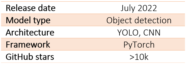
What is YOLOv7?
What Makes YOLO popular for object detection?
YOLO stands for “You Only Look Once”; it is a popular family of real-time object detection algorithms. The original YOLO object detector was first released in 2016. It was created by Joseph Redmon, Ali Farhadi, and Santosh Divvala. At release, this architecture was much faster than other object detectors and became state-of-the-art for real-time Computer Vision applications.
High mean Average Precision (mAP)
YOLO (You Only Look Once) has gained popularity in the field of object detection due to several key factors. making it ideal for real-time applications. Additionally, YOLO achieves higher mean Average Precision (mAP) than other real-time systems, further enhancing its appeal.
High detection accuracy
Another reason for YOLO's popularity is its high detection accuracy. It outperforms other state-of-the-art models with minimal background errors, making it reliable for object detection tasks.
YOLO also demonstrates good generalization capabilities, especially in its newer versions. It exhibits better generalization for new domains, making it suitable for applications that require fast and robust object detection. For example, studies comparing different versions of YOLO have shown improvements in mean average precision for specific tasks like the automatic detection of melanoma disease.
An open-source algorithm
Furthermore, YOLO's open-source nature has contributed to its success. The community's continuous improvements and contributions have helped refine the model over time.
YOLO's outstanding combination of speed, accuracy, generalization, and open-source nature has positioned it as the leading choice for object detection in the tech community. Its impact in the field of real-time Computer Vision cannot be understated.
YOLO architecture
The YOLO architecture shares similarities with GoogleNet, featuring convolutional layers, max-pooling layers, and fully connected layers.
).](https://res.cloudinary.com/practicaldev/image/fetch/s--toFb3X3o--/c_limit%2Cf_auto%2Cfl_progressive%2Cq_auto%2Cw_800/https://cdn-images-1.medium.com/max/2614/0%2AP2UBhFj_oTtoVup-.png)
The architecture follows a streamlined approach to object detection and work as follows:
Starts by resizing the input image to a fixed size, typically 448x448 pixels.
This resized image is then passed through a series of convolutional layers, which extract features and capture spatial information.
The YOLO architecture employs a 1x1 convolution followed by a 3x3 convolution to reduce the number of channels and generate a cuboidal output.
The Rectified Linear Unit (ReLU) activation function is used throughout the network, except for the final layer, which utilizes a linear activation function.
To improve the model's performance and prevent overfitting, techniques such as batch normalization and dropout are employed. Batch normalization normalizes the output of each layer, making the training process more stable. Dropout randomly ignores a portion of the neurons during training, which helps prevent the network from relying too heavily on specific features.
How does YOLO object detection work?
In terms of how YOLO performs object detection, it follows a four-step approach:
)](https://res.cloudinary.com/practicaldev/image/fetch/s--ytmJ9tqd--/c_limit%2Cf_auto%2Cfl_progressive%2Cq_auto%2Cw_800/https://cdn-images-1.medium.com/max/2216/0%2A3PIFIVlYFD0iWfaa.jpg)
First, the image is divided into grid cells (SxS) responsible for localizing and predicting the object's class and confidence values.
Next, bounding box regression is used to determine the rectangles highlighting the objects in the image. The attributes of these bounding boxes are represented by a vector containing probability scores, coordinates, and dimensions.
Intersection Over Unions (IoU) is then employed to select relevant grid cells based on a user-defined threshold.
Finally, Non-Max Suppression (NMS) is applied to retain only the boxes with the highest probability scores, filtering out potential noise.
Overview of the YOLOv7 model
)](https://res.cloudinary.com/practicaldev/image/fetch/s--cuRO3hXR--/c_limit%2Cf_auto%2Cfl_progressive%2Cq_auto%2Cw_800/https://cdn-images-1.medium.com/max/2000/0%2AS9d2tHHY0egJkD_n.png)
Compared to its predecessors, YOLOv7 introduces several architectural reforms that contribute to improved performance. These include:
● Architectural reform:
Model scaling for concatenation-based models allows the model to meet the needs of different inference speeds.
E-ELAN (Extended Efficient Layer Aggregation Network) which allows the model to learn more diverse features for better learning.
● Trainable Bag-of-Freebies (BoF) improving the model’s accuracy without increasing the training cost using:
Planned re-parameterized convolution.
Coarse for auxiliary and fine for lead loss.
YOLO v7 introduces a notable improvement in resolution compared to its predecessors. It operates at a higher image resolution of 608 by 608 pixels, surpassing the 416 by 416 resolution employed in YOLO v3. By adopting this higher resolution, YOLO v7 becomes capable of detecting smaller objects more effectively, thereby enhancing its overall accuracy.
These enhancements result in a 13.7% higher Average Precision (AP) on the COCO dataset compared to YOLOv6.
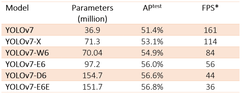
Parameters and FPS
The YOLOv7 model has six versions with varying parameters and FPS (Frames per Second) performance. Here are the details:
Step by step: Fine tune a pre-trained YOLOv7 model using Ikomia API
With the dataset of aerial images that you downloaded, you can train a custom YOLO v7 model using the Ikomia API.
Step 1: import
from ikomia.dataprocess.workflow
import Workflowfrom ikomia.utils import ik
“Workflow” is the base object to create a workflow. It provides methods for setting inputs such as images, videos, and directories, configuring task parameters, obtaining time metrics, and accessing specific task outputs such as graphics, segmentation masks, and texts.
“ik” is an auto-completion system designed for convenient and easy access to algorithms and settings.
Step 2: create workflow
We initialize a workflow instance. The “wf” object can then be used to add tasks to the workflow instance, configure their parameters, and run them on input data.
wf = Workflow()
Step 3: add the dataset loader
The downloaded dataset is in YOLO format, which means that for each image in each folder (test, val, train), there is a corresponding .txt file containing all bounding box and class information associated with airplanes. Additionally, there is a _darknet.labels file containing all class names. We will use the dataset_yolo module provided by Ikomia API to load the custom data and annotations.
dataset = wf.add_task(ik.dataset_yolo(
    dataset_folder="path/to/aerial/dataset/train",
    class_file="path/to//aerial/dataset/train/_darknet.labels")
)
Step 4: add the YOLOv7 model and set the parameters
We add a train_yolo_v7 task to train our custom YOLOv7 model. We also specify a few parameters:
yolo = wf.add_task(ik.train_yolo_v7(
    batch_size="4",
    epochs="10",
    output_folder="path/to/output/folder"),
    auto_connect=True
)
batch_size: Number of samples processed before the model is updated.
epochs: Number of complete passes through the training dataset.
train_imgz: Input image size during training.
test_imgz: Input image size during testing.
dataset_spilt_ratio: the algorithm divides automatically the dataset into train and evaluation sets. A value of 0.9 means the use of 90% of the data for training and 10% for evaluation.
The “auto_connect=True ” argument ensures that the output of the dataset_yolo task is automatically connected to the input of the train_yolo_v7 task.
Step 5: apply your workflow to your dataset
Finally, we run the workflow to start the training process.
wf.run()
You can monitor the progress of your training using tools like Tensorboard or MLflow.
Once the training is complete, the train_yolo_v7 task will save the best model in a folder named with a timestamp inside the output_folder. You can find your best.pt model in the weights folder of the timestamped folder.
Test your fine-tuned YOLOv7 model
First, we can run an aerial image on the pre-trained YOLOv7 model:
from ikomia.dataprocess.workflow import Workflow
from ikomia.utils.displayIO import display
from ikomia.utils import ik

# Initialize the workflow
wf = Workflow()

# Add an Object Detection algorithm
yolo = wf.add_task(ik.infer_yolo_v7(thr_conf="0.4"), auto_connect=True)

# Run on your image
wf.run_on(path="/path/to/aerial/dataset/test/airport_246_jpg.rf.3d892810357f48026932d5412fa81574.jpg")

# Inspect your results
display(yolo.get_image_with_graphics())
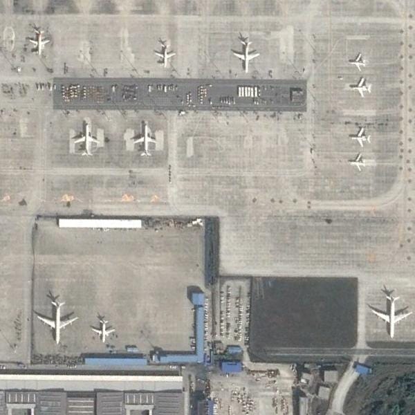
We can observe that the infer_yolo_v7 default pre-trained model doesn’t detect any plane. This is because the model has been trained on the COCO dataset, which does not contain aerial images of airports. As a result, the model lacks knowledge of what an airplane looks like from above.
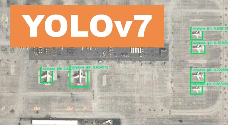
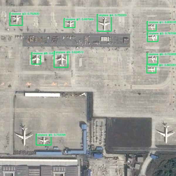
To test the model we just trained, we specify the path to our custom model using the ’model_weight_file’ argument. We then run the workflow on the same image we used previously.
# Use your custom YOLOv7 model
yolo = wf.add_task(ik.infer_yolo_v7(
    model_weight_file="path/to/output_folder/timestamp/weights/best.pt",
    thr_conf="0.4"),
    auto_connect=True
)
Conclusion
In this comprehensive guide, we have dived into the process of fine-tuning the YOLOv7 pre-trained model, empowering it to achieve higher accuracy when identifying specific object classes.
The Ikomia API serves as a game-changer, streamlining the development of Computer Vision workflows and enabling effortless experimentation with various parameters to unlock remarkable results.
For a deeper understanding of the API's capabilities, we recommend referring to the documentation. Additionally, don't miss the opportunity to explore the impressive roster of advanced algorithms available on Ikomia HUB, and take a spin with Ikomia STUDIO, a user-friendly interface that mirrors the API's features.

Top comments (0)