
Dynamic programming is a technique for solving problems, whose solution can be expressed recursively in terms of solutions of overlapping sub-problems. A gentle introduction to this can be found in How Does DP Work? Dynamic Programming Tutorial.
Memoization is an optimization process. In simple terms, we store the intermediate results of the solutions of sub-problems, allowing us to speed up the computation of the overall solution. The improvement can be reduced to an exponential time solution to a polynomial time solution, with an overhead of using additional memory for storing intermediate results.
Let's understand how dynamic programming works with memoization with a simple example.

This lesson was originally published at https://algodaily.com, where I maintain a technical interview course and write think-pieces for ambitious developers.
Fibonacci Numbers
You have probably heard of Fibonacci numbers several times in the past, especially regarding recurrence relations or writing recursive functions. Today we'll see how this simple example gives us a true appreciation of the power of dynamic programming and memoization.
Definition of Fibonacci Numbers
The nth Fibonacci number f(n) is defined as:
f(0) = 0                                       // base case
f(1) = 1                                       // base case
f(n) = f(n-1) + f(n-2)    for n>1              // recursive case
The sequence of Fibonacci numbers generated from the above expressions is:
0 1 1 2 3 5 8 13 21 34 ...
Pseudo-code for Fibonacci Numbers
When implementing the mathematical expression given above, we can use the following recursive pseudo-code attached.
Routine: f(n)
Output: Fibonacci number at the nth place

Base case:
1. if n==0 return 0
2. if n==1 return 1

Recursive case:
1. temp1 = f(n-1)
2. temp2 = f(n-2)
3. return temp1+temp2
The recursion tree shown below illustrates how the routine works for computing f(5) or fibonacci(5).
If we look closely at the recursive tree, we can see that the function is computed twice for f(3), thrice for f(2) and many times for the base cases f(1) and f(0). The overall complexity of this pseudo-code is therefore exponential O(2^n). We can very well see how we can achieve massive speedups by storing the intermediate results and using them when needed.
Memoization of Fibonacci Numbers: From Exponential Time Complexity to Linear Time Complexity
To speed things up, let's look at the structure of the problem. f(n) is computed from f(n-1) and f(n-2). As such, we only need to store the intermediate result of the function computed for the previous two numbers. The pseudo-code to achieve this is provided here.
The figure below shows how the pseudo-code is working for f(5). Notice how a very simple memoization technique that uses two extra memory slots has reduced our time complexity from exponential to linear (O(n)).
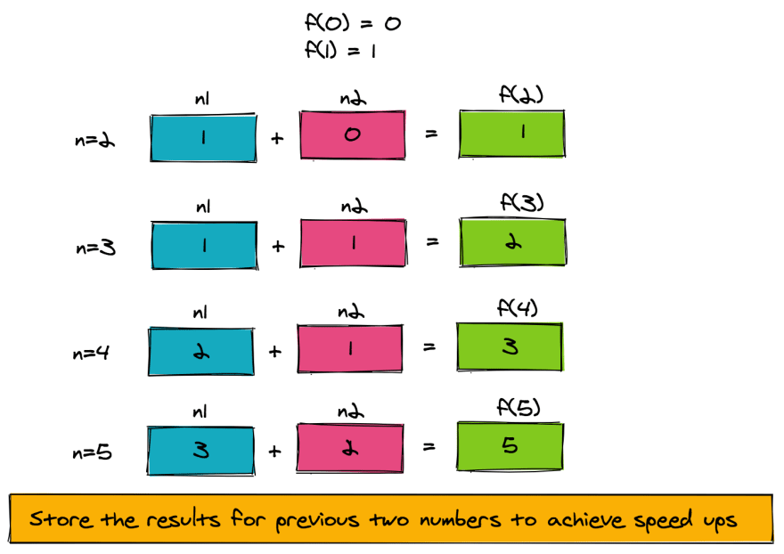
Routine: fibonacciFast
Input: n
Output: Fibonacci number at the nth place
Intermediate storage: n1, n2 to store f(n-1) and f(n-2) respectively

1. if (n==0) return 0
2. if (n==1) return 1
3. n1 = 1
4. n2 = 0
5. for 2 .. n
    a. result = n1+n2           // gives f(n)
    b.   n2 = n1                // set up f(n-2) for next number
    c.   n1 = result            // set up f(n-1) for next number
6. return result
Maximizing Rewards While Path Finding Through a Grid
Now that we understand memoization a little better, let's move on to our next problem. Suppose we have an m * n grid, where each cell has a "reward" associated with it. Let's also assume that there's a robot placed at the starting location, and that it has to find its way to a "goal cell". While it's doing this, it will be judged by the path it chooses. We want to get to the "goal" via a path that collects the maximum reward. The only moves allowed are "up" or "right".
Using a Recursive Solution
This awesome tutorial on recursion and backtracking tells you how to enumerate all paths through this grid via backtracking. We can use the same technique for collecting the "maximum reward" as well, via the following two steps:
1. Enumerate all paths on the grid, while computing the reward along each path
2. Select the path with the maximum reward
Let's look at how this code will work. The below illustration has a 3 x 3 grid. We've kept the grid small because the tree would otherwise be too long and too wide. The 3 x 3 grid only has 6 paths, but if you have a 4 x 4 grid, you'll end up with 20 paths (and for a 5 x 5 grid there would be 70):
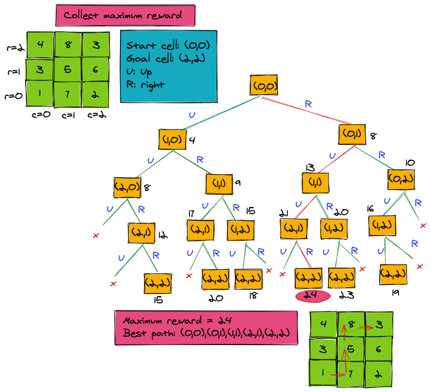
We can very well see that such a solution has exponential time complexity-- in other words, O(2^mn) -- and it's not very smart.
Dynamic Programming and Memoization
Let's try to come up with a solution for path-finding while maximizing reward, by using the following observation:
If the path with the maximum reward passes through cell (r, c), then it is also the best path from the start to (r, c), and the best path from (r, c) to goal.
This is the fundamental principle behind finding the optimum, or best path, that collects the maximum reward. We have broken down a large problem into two smaller sub-problems:
- Best path from start to
(r, c) - Best path from
(r, c)to goal
Combining the two will give us the overall optimal path. Since we don't know in advance which cells are a part of the optimal path, we'll want to store the maximum reward accumulated when moving from the start to all cells of the grid. The accumulated reward of the goal cell gives us the optimal reward. We'll use a similar technique to find the actual optimal path from start to goal.
Let's use a matrix array called reward that will hold the accumulated maximum reward from the start to each cell. Hence, we have the following matrices:
// input matrix where:
w[r, c]  = reward for individual cell (r, c)

// intermediate storage where:
reward[r, c] = maximum accumulated reward along the path from the start to cell (r, c)
Here is the recursive pseudo-code that finds the maximum reward from the start to the goal cell. The pseudo-code finds the maximum possible reward when moving up or right on an m x n grid. Let's assume that the start cell is (0, 0) and the goal cell is (m-1, n-1).
To get an understanding of the working of this algorithm, look at the figure below. It shows the maximum possible reward that can be collected when moving from start cell to any cell. For now, ignore the direction matrix in red.
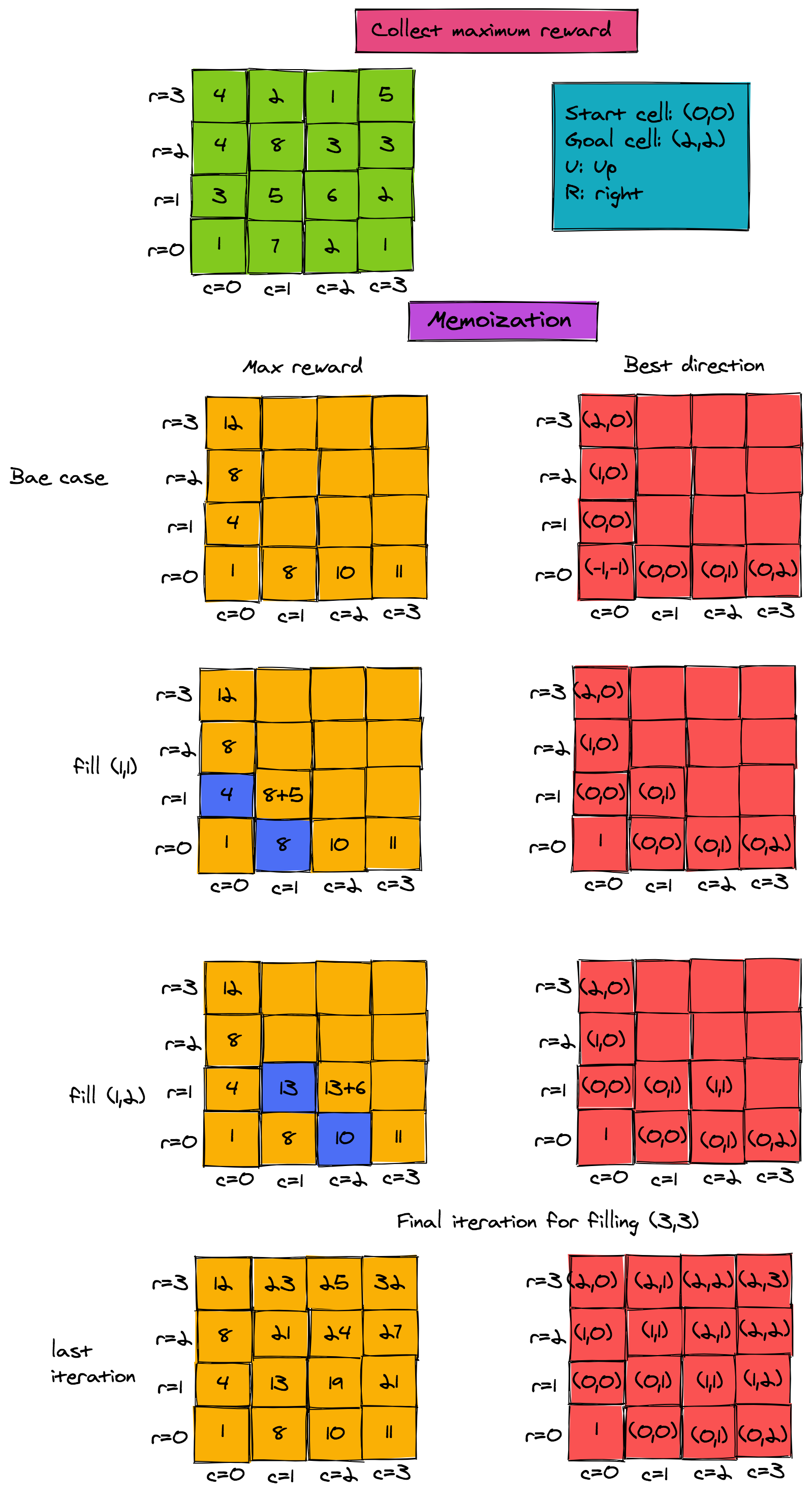
Routine: maximizeReward
Start cell coordinates: (0, 0)
Goal cell coordinates: (m-1, n-1)
Input: Reward matrix w of dimensions mxn

Base case 1:
// for cell[0, 0]
reward[0, 0] = w[0, 0]

Base case 2:
// zeroth col.  Can only move up
reward[r, 0] = reward[r-1, 0] + w[r, 0]  for r=1..m-1

Base case 3:
// zeroth row.  Can only move right
reward[0,c] = reward[0, c-1] + w[0, c] for c=1..n-1

Recursive case:
1. for r=1..m-1
    a. for c=1..n-1
        i. reward[r,c] = max(reward[r-1, c],reward[r, c-1]) + w[r, c]
2. return reward[m-1, n-1]           // maximum reward at goal state
Finding the Path via Memoization
Finding the actual path is also easy. All we need is an additional matrix, which stores the predecessor for each cell (r, c) when finding the maximum path. For example, in the figure above, when filling (1, 1), the maximum reward would be 8+5 when the predecessor in the path is the cell (0, 1). We need one additional matrix d that gives us the direction of the predecessor:
d[r,c] = coordinates of the predecessor in the optimal path reaching `[r, c]`.
The pseudo-code for filling the direction matrix is given by the attached pseudocode.
Routine: bestDirection
routine will fill up the direction matrix
Start cell coordinates: (0,0)
Goal cell coordinates: (m-1,n-1)
Input: Reward matrix w

Base case 1:
// for cell[0,0]
d[0,0] = (-1, -1)      //not used

Base case 2:
// zeroth col.  Can only move up
d[r,0] = (r-1, 0)   for r=1..m-1

Base case 3:
// zeroth row.  Can only move right
reward[0, c] = d[0,c-1] for c=1..n-1

Recursive case:
1. for r=1..m-1
    a. for c=1..n-1
        i. if reward[r-1,c] > reward[r,c-1])
                then d[r,c] = (r-1, c)
           else
                 d[r,c] = (r, c-1)
2. return d
Once we have the direction matrix, we can backtrack to find the best path, starting from the goal cell (m-1, n-1). Each cell's predecessor is stored in the matrix d.
If we follow this chain of predecessors, we can continue until we reach the start cell (0, 0). Of course, this means we'll get the path elements in the reverse direction. To solve for this, we can push each item of the path on a stack and pop them to get the final path. The steps taken by the pseudo-code are shown in the figure below.
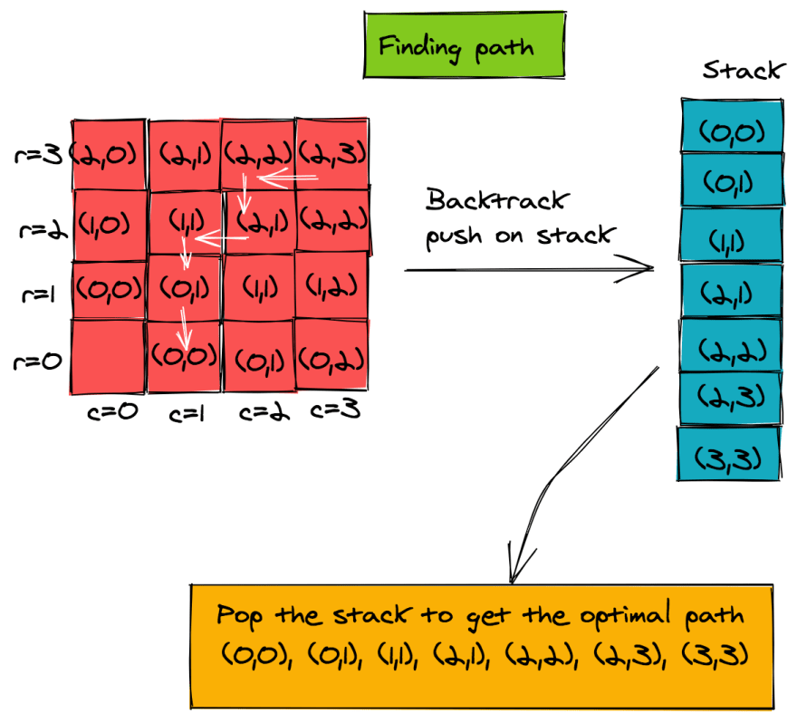
Routine: printPath
Input: direction matrix d
Intermediate storage: stack

// build the stack
1. r = m-1
2. c = n-1
3. push (r, c) on stack
4. while (r!=0 && c!=0)
    a. (r, c) = d[r, c]
    b. push (r, c) on stack
// print final path by popping stack
5. while (stack is not empty)
    a. (r, c) = stack_top
    b. print (r, c)
    c. pop_stack
Time Complexity of Path Using Dynamic Programming and Memoization
We can see that using matrices for intermediate storage drastically reduces the computation time. The maximizeReward function fills each cell of the matrix only once, so its time complexity is O(m * n). Similarly, the best direction also has a time complexity of O(m * n).
The printPath routine would print the entire path in O(m+n) time. Thus, the overall time complexity of this path finding algorithm is O(m * n). This means we have a drastic reduction in time complexity from O(2^mn) to O(m + n). This, of course, comes at a cost of additional storage. We need additional reward and direction matrices of size m * n, making the space complexity O(m * n). The stack of course uses O(m+n) space, so the overall space complexity is O(m * n).
Weighted Interval Scheduling via Dynamic Programming and Memoization
Our last example in exploring the use of memoization and dynamic programming is the weighted interval scheduling problem.
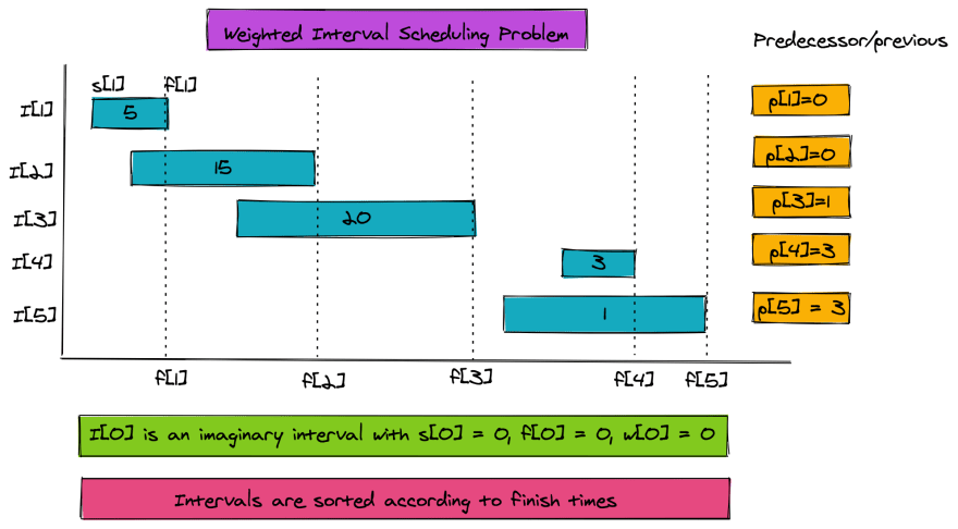
We are given n intervals, each having a start and finish time, and a weight associated with them. Some sets of intervals overlap and some sets do not. The goal is to find a set of non-overlapping intervals to maximize the total weight of the selected intervals. This is a very interesting problem in computer science, as it is used in scheduling CPU tasks, and in manufacturing units to maximize profits and minimize costs.
Problem Parameters
The following are the parameters of the problem:
1. n = total intervals.  We'll use an additional zeroth interval for base case.
2. Each interval has a start time and a finish time.
    Hence there are two arrays s and f, both of size (n+1)
    s[j] < f[j] for j=1..n and s[0] = f[0] = 0
3. Each interval has a weight w, so we have a weight array w.  w[j] >0  for j=1..n and w[0]=0
4. The interval array is sorted according to finish times.
Additionally we need a predecessor array p:
6. p[j] = The non-overlapping interval with highest finish time which is less than f[j].
            p[j] is the interval that finishes before p[j]
To find p[j], we only look to the left for the first non-overlapping interval. The figure below shows all the problem parameters.
A Recursive Expression for Weighted Interval Scheduling
As mentioned before, dynamic programming combines the solutions of overlapping sub-problems. Such a problem, the interval scheduling for collecting maximum weights, is relatively easy.
For any interval j, the maximum weight can be computed by either including it or excluding it. If we include it, then we can compute the sum of weights for p[j], as p[j] is the first non-overlapping interval that finishes before I[j]. If we exclude it, then we can start looking at intervals j-1 and lower. The attached is the recursive mathematical formulation.
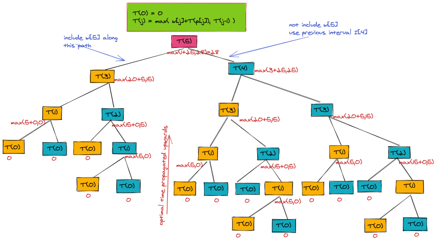
The below figure shows the recursion tree when T(5) is run.
Routine: T(j)
Input: s, f and w arrays (indices 0..n).  Intervals are sorted according to finish times
Output: Maximum accumulated weight of non-overlapping intervals

Base case:
1. if j==0 return 0

Recursive case T(j):
1. T1 = w[j] + T(p[j])
2. T2 = T(j-1)
3. return max(T1,T2)
Scheduling via Dynamic Programming and Memoization
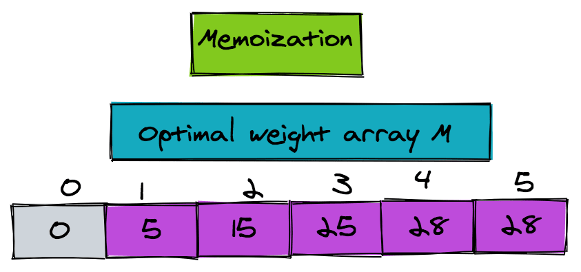
From the recursion tree, we can see that the pseudo-code for running the T function has an exponential time complexity of O(2$^n$). From the tree, we can see how to optimize our code. There are parameter values for which T is computed more than once-- examples being T(2), T(3), etc. We can make it more efficient by storing all intermediate results and using those results when needed, rather than computing them again and again. Here's the faster version of the pseudo-code, while using an additional array M for memoization of maximum weights up to nth interval.
Routine: TFast(j)
Input: f, s and w arrays (indices 0..n).  Intervals sorted according to finish times
Output: Maximum accumulated weight of non-overlapping intervals
Intermediate storage: Array M size (n+1) initialized to -1

Base case:
1. if j==0
    M[0] = 0;
    return 0

Recursive case Tfast(j):
1. if M[j] != -1            //if result is stored
    return M[j]             //return the stored result
1. T1 = w[j] + TFast[p[j]]
2. T2 = TFast[j-1]
3. M[j] = max(T1, T2)
4. return M[j]
The great thing about this code is that it would only compute TFast for the required values of j. The tree below is the reduced tree when using memoization. The values are still propagated from leaf to root, but there is a drastic reduction in the size of this tree.
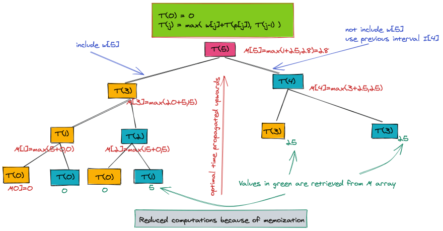
The figure shows the optimal weight array M:
Finding the Interval Set
There is one thing left to do-- find out which intervals make up the optimal set. We can use an additional array X, which is a Boolean array. X[j] indicates whether we included or excluded the interval j, when computing the max. We can fill up array X as we fill up array M. Let's change TFast to a new function TFastX to do just that.
We can retrieve the interval set using the predecessor array p and the X array. Below is the pseudo-code:
Routine: printIntervals
1. j=n
2. while (j>0)
    a. If X[j] == 1             //Is j to be included?
       i.     print j
       ii.    j = p[j]          //get predecessor of j
        else
            j = j-1
The whole process is illustrated nicely in the figure below. Note in this case too, the intervals are printed in descending order according to their finish times. If you want them printed in reverse, then use a stack like we did in the grid navigation problem. That change should be trivial to make.

Routine: TFastX(j)
Input: f,s and w arrays (indices 0..n).  Intervals sorted according to finish times
Output: Maximum accumulated weight of non-overlapping intervals
Intermediate storage: Array M size (n+1) initialized to -1,
                      Array X size (n+1) initialized to 0

Base case:
1. if j==0
M[0] = 0;
X[0] = 0
return 0

Recursive case TfastX(j):
1. if M[j] != -1            // if result is stored
return M[j]                 // return the stored result
1. T1 = w[j] + TFast[p[j]]
2. T2 = TFast[j-1]
3. if (T1 > T2)
        X[j] = 1                    // include jth interval else X[j] remains 0
4. M[j] = max(T1, T2)
5. return M[j]
Time Complexity of Weighted Interval Scheduling via Memoization
The time complexity of the memoized version is O(n). It is easy to see that each slot in the array is filled only once. For each element of the array, there are only two values to choose the maximum from-- thus the overall time complexity is O(n). However, we assume that the intervals are already sorted according to their finish times. If we have unsorted intervals, then there is an additional overhead of sorting the intervals, which would require O(n log n) computations.
Well, that's it for now. You can look at the Coin Change problem and Longest Increasing Subsequence for more examples of dynamic programming. I hope you enjoyed this tutorial as much as I did creating it!
This lesson was originally published at https://algodaily.com, where I maintain a technical interview course and write think-pieces for ambitious developers.

Top comments (2)
Nice explanations. I really liked the graphs.
Very nice article :-) Which software did you use for the graphs?