Document Classification: 7 pragmatic approaches for small datasets

This article was originally posted by Shahul ES on neptune.ml/blog where you can find more in-depth articles for machine learning practitioners.

---

Document or text classification is one of the predominant tasks in Natural language processing. It has many applications including news type classification, spam filtering, toxic comment identification, etc.

In big organizations the datasets are large and training deep learning text classification models from scratch is a feasible solution but for the majority of real-life problems your dataset is small and if you want to build your machine learning model you need to be smart.

In this article, I will talk about pragmatic approaches towards text representation which make document classification on small datasets doable.

Text Classification 101

The text classification workflow begins by cleaning and preparing the corpus out of the dataset. Then this corpus is represented by any of the different text representation methods which are then followed by modeling.

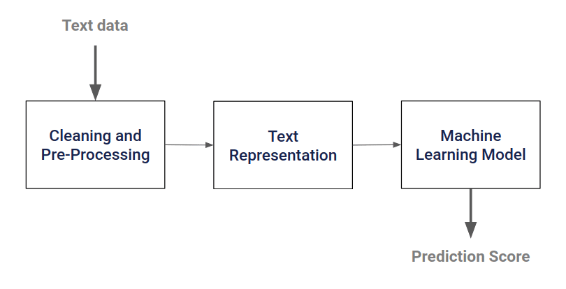
In this article, we will focus on the “Text Representation” step of this pipeline.

Example text classification dataset

We will use the data from Real or Not? NLP with disaster tweets kaggle competition. Here, the task is to predict which tweets are about real disasters and which ones are not.

If you want to follow the article step-by-step you may want to install all the libraries that I used for the analysis.

Let’s take a look at our data,

import pandas as pd

tweet= pd.read_csv('../input/nlp-getting-started/train.csv')
test=pd.read_csv('../input/nlp-getting-started/test.csv')

tweet.head(3)

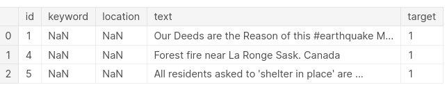
The data contains of id, keyword, location, text, and target which is binary. We will only consider the tweets to predict the target.

print('There are {} rows and {} columns in train'.format(tweet.shape[0],tweet.shape[1]))
print('There are {} rows and {} columns in test'.format(test.shape[0],test.shape[1]))

The training dataset has less than 8000 tweets. That, combined with the fact that tweets are 280 characters tops make it a tricky, small(ish) dataset.

Text data preparation

Before we get into any NLP task, we need to do some data preprocessing and basic cleaning. It is not a focus of this article but if you want to read more about this step check out this article.

In short, we will:

• Tokenize: the process by which sentences are converted to a list of tokens or words.
• Remove stopwords: drop words like ‘a’ or ‘the’
• Lemmatize: reduce the inflectional forms of each word into a common base or root (“studies”, “studying” -> “study”).

def preprocess_news(df):
    '''Function to preprocess and create corpus'''
    new_corpus=[]

    lem=WordNetLemmatizer()
    for text in df["question_text"]:
        words=[w for w in word_tokenize(text) if (w not in stop)]

        words=[lem.lemmatize(w) for w in words]

        new_corpus.append(words)
    return new_corpus

corpus=preprocess_news(df)

Now, let’s see how to represent this corpus so that we can feed this into any machine learning algorithm.

Text Representation

Text cannot be used directly as input to a machine learning model but needs to be represented in the numeric format first. This is known as text representation.

Countvectorizer

Countvectorizer provides an easy method to vectorize and represent a collection of text documents. It tokenizes the input text and builds a vocabulary of known words and then represents the documents using this vocabulary.

Let’s understand it by using an example,

text = ["She sells seashells in the seashore"]
# create the transform
vectorizer = CountVectorizer()
# tokenize and build vocab
vectorizer.fit(text)
# summarize
print(vectorizer.vocabulary_)
# encode document
vector = vectorizer.transform(text)
# summarize encoded vector
print(vector.shape)
print(type(vector))
print(vector.toarray())

You can see that the Coutvectorizer has built a vocabulary out of the given text and then represented the words using a numpy sparse matrix. We can try and transfer another text using this vocabulary and observe the output to get a better understanding.

vector=vectorizer.transform(["I sell seashells in the seashore"])
vector.toarray()

You can see that:

• The index positions 3 and 4 have zeroes meaning that these two words are not present in our vocabulary and all other positions have 1 meaning that these words are present in our vocabulary. The corresponding words missing from the vocabulary are “sells” and “she”. Now that you understand how Coutvectorizer works, we can fit and transform our corpus using it.

vec=CountVectorizer(max_df=10,max_features=10000)
vec.fit(df.question_text.values)
vector=vec.transform(df.question_text.values)

You should know that Countvectorizer has a few important parameters that you should adjust to your problem:

• max_features: build a vocabulary that only considers the top n tokens ordered by term frequency across the corpus.
• min_df: When building the vocabulary ignore terms that have a token frequency strictly lower than the given threshold
• max_df: When building the vocabulary ignore terms that have a token frequency strictly higher than the given threshold.

What usually helps with selecting reasonable values (or ranges for hyperparameter optimization methods) is good exploratory data analysis. Check out my other article to read about it.

TfidfVectorizer

One issue with Countvectorizer is that common words like “the” will appear many times (unless you remove them at the preprocessing stage) and these words are not actually important. One popular alternative is Tfidfvectorizer. It is an acronym for Term frequency-inverse document frequency.

• Term Frequency: This summarizes how often a given word appears within a document.
• Inverse Document Frequency: This downscales words that appear a lot across documents.

Let’s look at an example:

from sklearn.feature_extraction.text import TfidfVectorizer
# list of text documents
text = ["She sells seashells by the seashore","The sea.","The seashore"]
# create the transform
vectorizer = TfidfVectorizer()
# tokenize and build vocab
vectorizer.fit(text)
# summarize
print(vectorizer.vocabulary_)
print(vectorizer.idf_)
# encode document
vector = vectorizer.transform([text[0]])
# summarize encoded vector
print(vector.shape)
print(vector.toarray())

The vocabulary again consists of 6 words and the inverse document frequency is calculated for each word, assigning the lowest score to “the” which occurred 4 times.

Then the scores are normalized between 0 and 1 and this text representation can be used as input into any machine learning model.

Word2vec

The big issue with the above approaches is that the context of the word is lost when representing it. Word embeddings provide a much better representation of the words in NLP by encoding some context information. It provides a mapping from a word to a corresponding n-dimensional vector.

Word2Vec was developed at Google by Tomas Mikolov, et al. and uses a shallow neural network to learn word embeddings. The vectors are learned by understanding the context in which the word occurs. Specifically, it looks at co-occurring words.

Given below is the co-occurrence matrix for the sentence “The cat sat on the mat”.

Word2vec is composed of two different models:

• Continuous Bag of Words (CBOW) model can be thought of as learning word embeddings by training a model to predict a word given its context.
• Skip-Gram model is the opposite, learning word embeddings by training a model to predict context given a word. The basic idea of word embedding is words that occur in similar context tend to be closer to each other in vector space. Let’s check how to implement word2vec in python.

import gensim
from gensim.models import Word2Vec

model = gensim.models.Word2Vec(corpus, 
                               min_count = 1, size = 100, window = 5)

Now you have created your word2vec model, some of the important parameters that you can actually change and observe the differences are,

• size: this indicates the embedding size of the resulting vector for each word.
• min_count: When building the vocabulary ignore terms that have a document frequency strictly lower than the given threshold
• window: The number of words surrounding the word is considered when building the representation. Also known as the window size. In this article, we focus on pragmatic approaches for small datasets and we will use pre-trained word vectors instead of training vectors from our corpus. This method is guaranteed to yield better performance.

First, you will have to download the trained vectors from here. Then you can load the vectors using gensim.

from  gensim.models.KeyedVectors import load_word2vec_format

def load_word2vec():
    word2vecDict = load_word2vec_format(
        '../input/word2vec-google/GoogleNews-vectors-negative300.bin',
        binary=True, unicode_errors='ignore')
    embeddings_index = dict()
    for word in word2vecDict.wv.vocab:
        embeddings_index[word] = word2vecDict.word_vec(word)

    return embeddings_index

Let’s check the embedding,

w2v_model=load_word2vec()
w2v_model['London'].shape

You can see that the word is represented using a 300-dimensional vector. So every word in your corpus can be represented like this and this embedding matrix is used to train your model.

FastText

Now, let’s learn about fastText which is an extremely useful module available in gensim. FastText has been developed by Facebook and yields great performance and speed in text classification tasks.

It supports both Continuous Bag of Words and Skip-Gram models. The main difference between previous models and FastText is that it breaks the word in several n-grams.

Let’s take the word orange for example.

The trigrams of word orange are,org,ran,ang,nge(ignoring the starting and ending boundaries of the word).

The word embedding vector (text representation)for orange will be the sum of these n-grams. Rare words or typos can now be properly represented since it is highly likely that some of their n-grams also appears in other words.

For example, for a word like stupedofantabulouslyfantastic, which might never have been in any corpus, gensim might return any two of the following solutions: a zero vector or a random vector with low magnitude.

FastText, however, can produce better vectors by breaking the word into chunks and using the vectors for those chunks to create a final vector for the word. In this particular case, the final vector might be closer to the vectors of fantastic and fantabulous.

Again, we will use a pre-trained model rather than training our own word embeddings.

For this, you can download pre-trained vectors from here.

Each line of this file contains a word and it’s a corresponding n-dimensional vector. We will create a dictionary using this file for mapping each word to its vector representation.

from gensim.models import FastText 

def load_fasttext():

    print('loading word embeddings...')
    embeddings_index = {}
    f = open('../input/fasttext/wiki.simple.vec',encoding='utf-8')
    for line in tqdm(f):
        values = line.strip().rsplit(' ')
        word = values[0]
        coefs = np.asarray(values[1:], dtype='float32')
        embeddings_index[word] = coefs
    f.close()
    print('found %s word vectors' % len(embeddings_index))

    return embeddings_index

embeddings_index=load_fastext()

Let’s check the embedding for a word,

embeddings_index['london'].shape

GloVe ( Global vectors for word representation)

GloVe stands for global vectors for word representation. It is an unsupervised learning algorithm developed by Stanford. The basic idea of GloVe is to derive a semantic relationship between words using a co-occurrence matrix. The idea is very similar to word2vec but there are slight differences. Go here to read more.

For this, we will use pre-trained glove vectors which are trained on large corpora. This is guaranteed to perform better in almost any situation.You can download it from here.

After downloading we can load our pre-trained word model. Before that, you should understand the format in which it is made available. Each line contains a word and its corresponding n-dimensional vector representation. Like this,

So, to use this you should first prepare a dictionary that contains the mapping between word and corresponding vector. This can be called an embedding dictionary.

Let’s create one for our purpose.

def load_glove():
    embedding_dict = {}
    path = '../input/glove-global-vectors-for-word-representation/glove.6B.100d.txt'
    with open(path, 'r') as f:
        for line in f:
            values = line.split()
            word = values[0]
            vectors = np.asarray(values[1:], 'float32')
            embedding_dict[word] = vectors
    f.close()

    return embedding_dict


embeddings_index = load_glove()

Now, we have a dictionary containing every word in the glove pre-trained vectors and their corresponding vector in a dictionary. Let’s check the embedding for a word.

embeddings_index['london'].shape

Universal Sentence Encoding

Till now we were dealing with representing words and these techniques are most useful for word-level operations. Sometimes we need to explore sentence level operations. These encoders are called sentence encoders.

A good sentence encoder is expected to encode sentences in such a way that the vectors of similar sentences have a minimal distance between them in the vector space.

For example,

• It is sunny today
• It is rainy today
• It is cloudy today. These sentences will be encoded and represented so that they are close to each other in the vector space.

Let’s move on and check how to implement universal sentence encoder and find similar sentences using it.

You can download the pertained vectors from here.

We will load the module using the TensorFlow hub.

module_url = "../input/universalsentenceencoderlarge4"
# Import the Universal Sentence Encoder's TF Hub module
embed = hub.load(module_url)

Next, we will create the embedding for each sentence in our list.

sentence_list=df.question_text.values.tolist()
sentence_emb=embed(sentence_list)['outputs'].numpy()

Here is an article to read more about universal sentence encoder.

Elmo, BERT, and others.

When using any of the above embedding methods one thing we forget about is the context in which the word was used. This is one of the main drawbacks of such word representation models.

For example, the word word “stick” will be represented using the same vector independent of the context in which it was used which doesn’t make much sense. With the recent developments in the field of NLP and models like BERT (bidirectional encoder representation from transformers), this has been made possible. Here is an article to read more.

Text Classification

In this section, we will prepare the embedding matrix which is passed to the Keras Embedding layer to learn text representations. You can use the same steps to prepare the corpus for any word-level embedding methods.

Let’s create a word index and fix a maximum sentence length, pad each sentence in our corpus using Keras Tokenizer and pad_sequences.

MAX_LEN=50
tokenizer_obj=Tokenizer()
tokenizer_obj.fit_on_texts(corpus)
sequences=tokenizer_obj.texts_to_sequences(corpus)

tweet_pad=pad_sequences(sequences,
                        maxlen=MAX_LEN,
                        truncating='post',
                        padding='post')

Let’s check the number of unique words in our corpus,

word_index=tokenizer_obj.word_index
print('Number of unique words:',len(word_index))

Using this word index dictionary and embedding dictionary you can create an embedding matrix for our corpus. This embedding matrix is passed on to the embedding layer of the neural network to learn word representations.

def prepare_matrix(embedding_dict, emb_size=300):
    num_words = len(word_index)
    embedding_matrix = np.zeros((num_words, emb_size))

    for word, i in tqdm(word_index.items()):
        if i > num_words:
            continue

    emb_vec = embedding_dict.get(word)
    if emb_vec is not None:
        embedding_matrix[i] = emb_vec

    return embedding_matrix

We can define our neural network and pass this embedding index to the Embedding layer of the network. We pass the vectors onto the Embedding layer and set trainable=False to prevent the weights from being updated.

def new_model(embedding_matrix):
    inp = Input(shape=(MAX_LEN,))

    x = Embedding(num_words, embedding_matrix.shape[1], weights=[embedding_matrix],
                  trainable=False)(inp)

    x = Bidirectional(
        LSTM(60, return_sequences=True, name='lstm_layer', 
             dropout=0.1, recurrent_dropout=0.1))(x)

    x = GlobalAveragePool1D()(x)
    x = Dense(1, activation="sigmoid")(x)
    model = Model(inputs=inp, outputs=x)

    model.compile(loss='binary_crossentropy',
                  optimizer='adam',
                  metrics=['accuracy'])

    return model

For example, to run the model using word2vec embeddings,

embeddings_index=load_word2vec()
embedding_matrix=prepare_matrix(embeddings_index)
model=new_model(embedding_matrix)

history=model.fit(X_train,y_train,
                  batch_size=8,
                  epochs=5,
                  validation_data=(X_test,y_test),
                  verbose=2)

You can call your desired type of embeddings and follow the same steps to implement any of them.

Comparison

So which text classification method worked best in our example problem?

You can use Neptune to compare the performance of our model using different embeddings by simply setting up an experiment.

Glove embeddings performed a little better in test sets when compared to the other two embeddings. You may be able to get better results by doing extensive cleaning on the data and tuning the model.

You can explore experiments here if you want to.

Final Thoughts

In this article, we discussed and implemented different feature representation methods for text classification that you can use for smaller datasets.

Hopefully, you will find them useful in your projects.

---

This article was originally posted on neptune.ml/blog where you can find more in-depth articles for machine learning practitioners.