Recognizing handwritten Arabic numbers is very simple for human beings, but it is still somewhat complicated for programs.
However, with the popularization of machine learning technology, it is not difficult to implement a program that can recognize handwritten numbers using over 10 lines of code. This is because there are too many machine learning models that can be directly used, such as TensorFlow and Caffe. There are ready-made installation packages available in Python, and for writing a program that recognizes numbers, a little over 10 lines of code is enough.
However, what I want to do is to completely implement such a program from scratch without using any third-party libraries. The reason for doing this is because you can deeply understand the principles of machine learning by implementing it yourself.
1 Model implementation
1.1 Principle
Those familiar with neural network regression algorithms can skip this section.
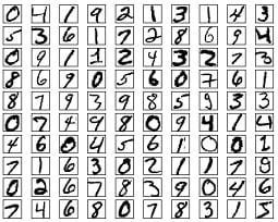
I have learned some basic concepts and decided to use regression algorithms. Firstly, I downloaded the famous MNIST dataset, which includes 60000 training samples and 10000 test samples. Each digital image is a 28 * 28 grayscale image, so the input can be considered as a 28 * 28 matrix or a 28 * 28=784 pixel value.
Here, a model is defined to determine an image number, with each model including the weight of each input, an intercept added, and finally normalized. Expression of the model:
Out5= sigmoid(X0*W0+ X1*W1+……X783*W783+bias)
X0 to X783 are 784 inputs, W0 to W783 are 784 weights, and bias is a constant. The sigmoid function can compress a large range of numbers into the (0,1) interval, which is called normalization.
For example, we use this set of weights and bias to determine the number 5, and expect the output to be 1 when the image is 5, and 0 when it is not 5. The training process then involves calculating the difference between the value of Out5 and the correct value (0 or 1) based on the input of each sample, and adjusting the weight and bias based on this difference. Transforming the formula is an effort to make (Out5- correct value) close to 0, which means minimizing the loss.
Similarly, 10 numbers require 10 sets of models, each with a different number to judge. After training, an image comes and is calculated using these 10 sets of models. If the result of the calculation is closer to 1, the image is considered to be a certain number.
1.2 Training
Following the above approach, use the SPL (Structured Process Language) of esProc to encode and implement:
    A   B   C
1   =file(“train-imgs.btx”).cursor@bi()
2   >x=[],wei=[],bia=[],v=0.0625,cnt=0
3   for 10  >wei.insert(0,[to(28*28).(0)]),
bia.insert(0,0.01)
4   for 50000   >label=A1.fetch(1)(1)
5       >y=to(10).(0), y(label+1)=1,x=[]
6       >x.insert(0,A1.fetch(28*28))    >x=x.(~/255)
7       =wei.(~**x).(~.sum()) ++ bia
8       =B7.(1/(1+exp(-~)))
9       =(B8–y)**(B8.(1-~))**B8
10      for 10  >wei(B10)=wei(B10)–x.(~*v*B9(B10)),
bia(B10)=bia(B10) - v*B9(B10)
11  >file(“MNIST_Model.btx”).export@b(wei),
file(“MNIST_Model.btx”).export@ba(bia)
No need to search anymore. All the code for training the model is here and no third-party libraries are used. Let’s analyze it below:
A1, use a cursor to import MNIST training samples. This is the format I have converted and can be directly accessed by esProc;
A2, define variables: input x, weight wei, training speed v, etc;
A3, B3, initialize 10 sets of models (each with 784 weights and 1 bias);
A4, loop 50000 samples for training, and train 10 models simultaneously;
B4, fetch the label, i.e, what the image is;
B5, calculate the correct 10 outputs and save them to variable y;
B6, get 28 * 28 pixels of this image as input, and C6 divides each input by 255 for normalization;
B7, calculate X0*W0+ X1*W1+……X783*W783+bias
B8,calculate sigmoid(B7)
B9, calculate the partial derivative, or gradient, of B8;
B10, C10, adjust the parameters of 10 models in a cyclic manner based on the values of B9;
A11, after training, save the model to a file.
1.3 Test
Test the success rate of this model and write a testing program using SPL:
    A   B   C
1   =file(“MNIST_Model.btx”).cursor@bi()    =[0,1,2,3,4,5,6,7,8,9]
2   >wei=A1.fetch(10),bia=A1.fetch(10)
3   >cnt=0
4   =file(“test-imgs.btx”).cursor@bi()
5   for 10000   >label=A4.fetch(1)(1)
6       >x=[]
7       >x.insert(0,A4.fetch(28*28))    >x=x.(~/255)
8       =wei.(~**x).(~.sum()) ++ bia
9       =B8.(round(1/(1+exp(-~)), 2))
10      =B9.pmax()
11      if label==B1(B10)   >cnt=cnt+1
12  =A1.close()
13  =output(cnt/100)
Running the test, the accuracy rate reached 91.1%, and I am very satisfied with this result. After all, this is only a single-layer model, and the accuracy rate I obtained using TensorFlow’s single-layer model is also slightly over 91%. Let’s parse the code below:
A1, import the model file;
A2, extract the model into variables;
A3, counter initialization (used to calculate success rate);
A4, import MNIST test samples, this file format is what I have converted;
A5, loop through 10000 samples for testing;
B5, get the label;
B6, clear input;
B7, fetch 28*28 pixels of this image as input, divide each input by 255 for normalization;
B8, calculate X0*W0+ X1*W1+……X783*W783+bias
B9, calculate sigmoid (B7)
B10, obtain the maximum value, which is the most likely number;
B11, add one to the correct measurement counter;
A12, A13, end of testing, close file, output accuracy.
1.4 Optimization
The optimization here is not about continuing to improve accuracy, but about improving the speed of training. Readers who want to improve the accuracy can try these methods:
Add a convolutional layer;
Do not use fixed values for learning speed, but decrease with the number of training sessions;
Do not use all zeros for the initial value of weight, and use normal distribution;
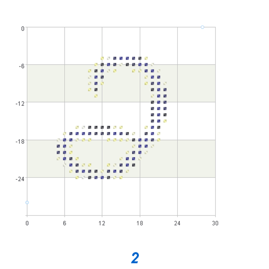
I don’t think pursuing accuracy alone is meaningful because some images in the MNIST dataset are inherently problematic, and even human may not necessarily recognize what number it is. I used esProc to display several incorrect images, all of which were written very irregularly. It is difficult to see that the image below is 2.
The key point is to improve the training speed by using parallelism or clustering. Implementing parallelism using SPL language is simple, as long as you use the fork keyword and slightly modify the above code.
    A   B   C   D
1   =file(“train-imgs.btx”).cursor@bi()
2   >x=[],wei=[],bia=[],v=0.0625,cnt=0  >mode=to(0,9)
3       >wei=to(28*28).(0)
4   fork mode   =A1.cursor()
5       for 50000   >label=B4.fetch(1)(1)   >y=1,x=[]
6           if label!=A4    >y=0
7           >x.insert(0,B4.fetch(28*28))    >x=x.(~/255)
8           =(wei**x).sum() + bia
9           =1/(1+exp(-C8))
10          =(C9-y)*((1-C9))*C9
11          >wei=wei–x.(~*v*C10),
bia=bia- v*C10
12      return wei,bia
13  =movefile(file(“MNIST_Model.btx”))
14  for 10  >file(“MNIST_Model.btx”).export@ba([A4(A15)(1)])
15  for 10  >file(“MNIST_Model.btx”).export@ba([A4(A16)(2)])
After using parallelism, the training time was reduced by almost half, and the code did not make too many modifications.
2 Why is it SPL language?
The use of SPL language may be a bit uncomfortable in the early stages, and it will become more and more convenient when you use more:
Support set operations, such as the multiplication of 784 inputs and 784 weights used in the example, simply write a **. If using Java or C, you need to implement it yourself.
The input and output of data is very convenient, making it easy to read and write files.
Debugging is very convenient, all variables are visually visible, which is better than Python.
It can be calculated step by step, and with changes, there is no need to start from the beginning. Java and C cannot do this, while Python can, but it is not convenient. esProc only needs to click on the corresponding cell to execute.
Implementing parallelism and clustering is very convenient and does not require too much development workload.
Support calling and being called. esProc can call third-party Java libraries, and Java can also call the code of esProc. For example, the above code can be called by Java to achieve an automatic verification code filling function.
This programming language is the most suitable for mathematical calculations.
Original : http://c.raqsoft.com/article/1688608216616
SPL Source code: http://c.raqsoft.com/article/1688608216616

Top comments (0)