Evaluation Metrics: Machine Learning Models 🤖🐍

Evaluation metrics are crucial in assessing the performance of machine learning models. These metrics help us understand how well our models are performing and where they might need improvement. In this post, we'll dive into evaluation metrics for two primary types of machine learning tasks: regression and classification. We'll also provide code examples using scikit-learn and its datasets.

What are Evaluation Metrics?

Evaluation metrics are quantitative measures used to evaluate the performance of machine learning models. They provide insights into how well the model is making predictions and help in comparing different models to select the best one for a given task.

Regression vs. Classification

• Regression: This involves predicting a continuous value. Examples include predicting house prices, stock prices, or temperature.
• Classification: This involves predicting a discrete label. Examples include classifying emails as spam or not spam, identifying the species of an iris flower, or detecting fraudulent transactions.

Regression Evaluation Metrics

1. Mean Absolute Error (MAE)
The Mean Absolute Error is the average of the absolute differences between predicted and actual values.
Formula : MAE = (1/n) * Σ|y_i - ŷ_i|

from sklearn.metrics import mean_absolute_error
from sklearn.datasets import load_boston
from sklearn.model_selection import train_test_split
from sklearn.linear_model import LinearRegression

# Load dataset
data = load_boston()
X, y = data.data, data.target

# Split data
X_train, X_test, y_train, y_test = train_test_split(X, y, test_size=0.2, random_state=42)

# Train model
model = LinearRegression()
model.fit(X_train, y_train)

# Predict
y_pred = model.predict(X_test)

# Evaluate
mae = mean_absolute_error(y_test, y_pred)
print(f'Mean Absolute Error: {mae}')

2. Mean Squared Error (MSE)
The Mean Squared Error is the average of the squared differences between predicted and actual values.

Formula: MSE = (1/n) * Σ(y_i - ŷ_i)^2

from sklearn.metrics import mean_squared_error

# Evaluate
mse = mean_squared_error(y_test, y_pred)
print(f'Mean Squared Error: {mse}')

3. Root Mean Squared Error (RMSE)
The Root Mean Squared Error is the square root of the average of the squared differences between predicted and actual values.

Formula: RMSE = √((1/n) * Σ(y_i - ŷ_i)^2)

import numpy as np

# Evaluate
rmse = np.sqrt(mse)
print(f'Root Mean Squared Error: {rmse}')

4. R-squared (R²)
R-squared is the proportion of the variance in the dependent variable that is predictable from the independent variables.

Formula:R² = 1 - (Σ(y_i - ŷ_i)^2 / Σ(y_i - ȳ)^2)

from sklearn.metrics import r2_score

# Evaluate
r2 = r2_score(y_test, y_pred)
print(f'R-squared: {r2}')

Classification Evaluation Metrics

1. Accuracy
Accuracy is the ratio of correctly predicted instances to the total instances.

Formula:Accuracy = (Number of correct predictions) / (Total number of predictions)

from sklearn.metrics import accuracy_score
from sklearn.datasets import load_iris
from sklearn.model_selection import train_test_split
from sklearn.ensemble import RandomForestClassifier

# Load dataset
data = load_iris()
X, y = data.data, data.target

# Split data
X_train, X_test, y_train, y_test = train_test_split(X, y, test_size=0.2, random_state=42)

# Train model
model = RandomForestClassifier()
model.fit(X_train, y_train)

# Predict
y_pred = model.predict(X_test)

# Evaluate
accuracy = accuracy_score(y_test, y_pred)
print(f'Accuracy: {accuracy}')

2. Precision
Precision is the ratio of correctly predicted positive observations to the total predicted positives.

Formula:Accuracy = (Number of correct predictions) / (Total number of predictions)

from sklearn.metrics import precision_score

# Evaluate
precision = precision_score(y_test, y_pred, average='weighted')
print(f'Precision: {precision}')

3. Recall
Recall is the ratio of correctly predicted positive observations to the all observations in actual class.

Formula:Recall = TP / (TP + FN)

from sklearn.metrics import recall_score

# Evaluate
recall = recall_score(y_test, y_pred, average='weighted')
print(f'Recall: {recall}')

4. F1 Score
The F1 Score is the weighted average of Precision and Recall.

Formula:F1 Score = 2 * (Precision * Recall) / (Precision + Recall)

from sklearn.metrics import f1_score

# Evaluate
f1 = f1_score(y_test, y_pred, average='weighted')
print(f'F1 Score: {f1}')

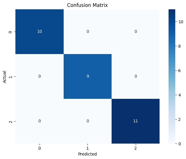
5. Confusion Matrix
The confusion matrix is a summary of prediction results on a classification problem. The correct and incorrect predictions are summarized with count values and broken down by each class.

Code Example:

from sklearn.metrics import confusion_matrix
import seaborn as sns
import matplotlib.pyplot as plt

# Evaluate
cm = confusion_matrix(y_test, y_pred)

# Plot
sns.heatmap(cm, annot=True, fmt='d', cmap='Blues')
plt.xlabel('Predicted')
plt.ylabel('Actual')
plt.show()

plot :

→ In this post, we explored various evaluation metrics for both regression and classification machine learning models. Understanding these metrics is crucial for interpreting model performance and making informed decisions to improve your models.

---

About Me:
🖇️LinkedIn
🧑‍💻GitHub