
In the previous series, we divulged a lot into Exploratory Data Analysis and how as a Data Scientist we have a lot of tools at our disposal to analyze and synthesize our data.
There is a popular misconception during the age of Big Data, is that because of the size and nature of data, the need for sampling is redundant. But on the contrary, because of the varying quality of data: the need for sampling is still prevalent.
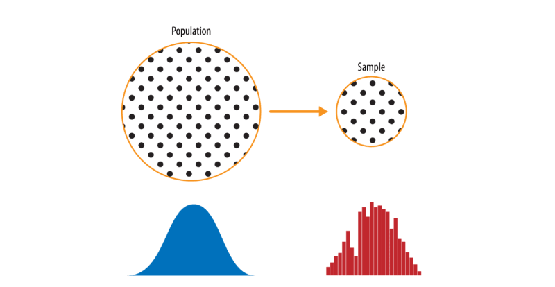
The lefthand side is the population which is assumed to follow an unknown distribution. The righthand side is the sample with an empirical distribution.
The process of picking up data from the lefthand side to the right-hand side is called sampling and which is the major concern in data science.
Random Sampling and Sample Bias
A sample is a subset of data from a larger data set, statisticians call this larger data set the population.
Random sampling is a process in which each available member of the population being sampled has an equal chance of being chosen for the sample at each draw.
Sampling can be done with replacement, in which observations are put back in the population after each draw for possible future reselection. Or it can be done without replacement, in which case observations, once selected, are unavailable for future draws.
What is Sample Bias?
It occurs when a sample drawn from the population was drawn in a nonrandom manner which resulted in a different distribution as compared to its population.
Bias
Statistical bias refers to measurement or sampling errors that are systematic and produced by the measurement or sampling process.
There is a large difference between Error from Bias and Error due to Random chance.
How to deal with Bias? - Random Selection
There are now a variety of methods to achieve representativeness, but at the heart of all of them lies random sampling.
Random sampling is not always easy. A proper definition of an accessible population is key.
In stratified sampling, the population is divided into stratas, and random samples are taken from each of them.
Selection Bias
Selection bias refers to the practice of selectively choosing data—consciously or unconsciously—in a way that leads to a conclusion that is misleading or ephemeral.
Selection bias occurs when you are data snooping, i.e extensive hunting for patterns inside data that suit your use-case.
Since the repeated review of large data sets is a key value proposition in data science, selection bias is something to worry about. A form of selection bias that a data scientist has to deal with is called Vast search effect.
If you repeatedly run different models and ask different questions with a large data set, you are bound to find something interesting. But is the result you found truly something interesting, or is it the chance outlier?
How to deal with this effect? The answer is by using a holdout set and sometimes more than one holdout set to validate against.
Sampling Distribution of Statistic
The term sampling distribution of a statistic refers to the distribution of some sample statistics over many samples drawn from the same population.
Much of the classical statistics is concerned with making inferences from small samples to a very large population.
Typically, a sample is drawn with the goal of measuring something (with a sample statistic) or modeling something (with a statistical or machine learning model).
Since our estimate or model is based on a sample, it might be in error, it might be different if we were to draw a different sample.
We are therefore interested in how different it might be, a key concern is sampling variability.
Note: It is important to distinguish between the distribution of the individual data points, known as the data distribution, and the distribution of a sample statistic, known as the sampling distribution.
The distribution of a sample statistic such as the mean is likely to be more regular and bell-shaped than the distribution of the data itself. The larger the sample the statistic is based on, the more this is true. Also, the larger the sample, the narrower the distribution of the sample statistic.
From an open-sourced Dataset- Wine Quality,
We are taking three samples from this data: a sample of 1,000 values, a sample of 1,000 means of 5 values, and a sample of 1,000 means of 20 values.
# Taking a Sample Data
sample_data = pd.DataFrame({
'total sulfur dioxide': data['total sulfur dioxide'].sample(1000), 'type': 'Data',
})

# Taking a mean of statistic for 5 samples

sample_mean_05 = pd.DataFrame({
    'total sulfur dioxide' : [data['total sulfur dioxide'].sample(5).mean() for _ in range(1000)],
    'type': 'Mean of 5'
})

# Taking mean of statistic for 20 samples

sample_mean_20 = pd.DataFrame({
    'total sulfur dioxide' : [data['total sulfur dioxide'].sample(20).mean() for _ in range(1000)],
    'type': 'Mean of 20'
})

results = pd.concat([sample_data, sample_mean_05, sample_mean_20])

g = sns.FacetGrid(results, col='type', col_wrap=1, height=2, aspect=2)
g.map(plt.hist, 'total sulfur dioxide', range=[0, 100], bins=40)
g.set_axis_labels('fixed acidity', 'Count')
g.set_titles('{col_name}')
The above code produces a FacetGrid consisting of three histograms, the first one being a data distribution, and second and third being sampling distribution.

The phenomenon we’ve just described is termed the Central limit theorem. It says that the means drawn from multiple samples will resemble the familiar bell-shaped normal curve.
The central limit theorem allows normal-approximation formulas like the t-distribution to be used in calculating sampling distributions for inference—that is, confidence intervals and hypothesis tests.
Standard Error
The standard error is a single metric that sums up the variability in the sampling distribution for a statistic.
The standard error can be estimated using a statistic based on the standard deviation s of the sample values, and the sample size n.

As the sample size increases, the standard error decreases, corresponding to what was observed in the above figure.
The approach to measuring standard error:
- Sample from an accessible population distribution
- For each sample, calculate the statistic (eg mean)
- Calculate the standard deviation of statistics from Step-2. Using this as an estimate for Standard Error.
In practice, this approach of collecting new samples to estimate the standard error is typically not feasible. Fortunately, it turns out that it is not necessary to draw brand new samples; instead, you can use bootstrap resamples.
In modern statistics, Bootstrap has become a standard way to estimate the standard error.
So this concludes Part-I, where I have divulged on Sample/Population Data dichotomy, Various types of bias in samples (Sample Bias), Ways to mitigate bias in our data, Central Limit Theorem and Standard Error.
Fin

Top comments (0)