Sentiment Analysis

Getting Started With Sentiment Analysis

It is the process of detecting positive or negative sentiment in text.
It is also referred to as opinion mining.
It is an approach to natural language processing (NLP) that identifies the emotional tone

behind a body of text.
It is vastly used by organizations to determine and categorize opinions about a produt, service or idea

Sentiment analysis involves the use of data mining, machine learning (ML), artificial intelligence

and computational linguistics to mine text for sentiment and subjective information.

Such information maybe classified as:

• positive
• neutral
• negative This classification is also known as polarity of a text. Graded Sentiment Analysis
• very positive
• positive
• Neutral
• Negative
• Very Negative This is also referred to as graded or fine-grained sentiment anlysis.

Types of Sentiment Analysis

• Intent-based - recognizes motivation behind a text
• Fine-grained - graded sentiment analysis
• Emotion-detection - allows detection of various emotions
• Aspect-based - anayses text to know particular aspects/features mentioned in all the polarity.

We will not dive into these types for now.

This in turn helps organizations to gather insights into real-time customer sentiment,

customer experience and brand reputation.

Generally these tools use text analytics to analyze online sources .

Benefits of sentiment analysis

• sorting data as scale
• real-time analysis
• consistent criteria

Steps involved in Sentiment Analysis

Sentiment analysis generally follows the following steps:

• Collect data - The text to be analyzed is identified and collected.
• Clean the data - The data is processed and cleaned to remove noise and parts of speech that don't have meaning relevant to the sentiment of the text.
• Extract features - A machine learning algorithm automatically extracts text features to identify negative or positive sentiment.
• Pick an ML model - A sentiment analysis tool scores the text using rule-based, automatic or hybrid ML model.
• Sentiment classification - Once a model is picked an used to analyze a piece of text, it assigns a sentiment score to the text including positive, negative of neutral.

Let's have a deep dive in sentiment analysis using an example

Step 1. Collect Data

We are going to used a data set from UCI Machine Learning Repository.

Let's start with importing the libraries that we will be using:
punkt is a data package that contains pre-trained models for tokenization.

# import the required packages and libraries
import numpy as np
import pandas as pd
import nltk
nltk.download('punkt')

loading the dataset

pd.set_option('display.max_colwith', None)
df = pd.read_csv('https://gist.githubusercontent.com/fmnobar/88703ec6a1f37b3eabf126ad38c392b8/raw/76b84540ccd4b0b207a6978eb7e9d938275886ff/imdb_labelled.csv')
df.head()

Output

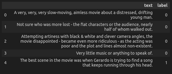
We can now see that there are only two columns text and label.
The label indicates the sentiment of the review

• 1 indicates a postive sentiment
• 0 indicates a negative sentiment. This thus indicates the polarity of the sentiment.

We now create a sample string, which is the first entry in the text column of the dataframe df.

sample = df.text[0]
sample

Output

Tokens and Bigrams

a. Tokens

A token is a single unit of meaning that can be identified in a text.
It is also known as a unigram.
Tokenization is the process of breaking down a text into individual tokens.
The functions that perform tokenization are called tokenizers.
This concept is implemented with the nltk.word_tokenize function.

• the function takes a string of text as input and returns a list of tokens.

• it splits the text into individual words and punctuation marks.
  Let's see an example the functions usage by tokenizing the sample text.

  sample_tokens = nltk.tokenize(sample)
  sample_tokens[:10] # view a list of elements upto the 10th token

Output

b. Bigrams

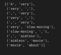
If we combine two unigrams/tokens we form a bigram.
A bigram is a pair of adjecent tokens in a text.
They are used to capture some of the context in which a particular word
or phrase appers.
They are used to build statistical models of language which are
sequences of n words/tokens.
By analyzing the frequency of different n-grams in a large corpus of text,
NLP systems can learn to predict the probability of dofferen words occuring in a particular context.

bigrams are implememted with the nltk.bigrams function

Let's see this in action

sample_bitokes = list(nltk.bigrams(sample_tokens))

# Return the first 10 bigrams
sample_bitokens[:10]

Output

Frequency Distribution

Refers to the count or proportion of words or prases asscociated with positive or negative sentiment.
It basically counts the occurrence of each sentiment-bearing word/phrase
and then calculate the frequency distribution.

implemented using the nltk.FreqDist function

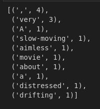
What are the top 10 most frequently used tokens in our sample?

sample_freqdist = nltk.FreqDist(sample_tokens)

# Return the top 10 most frequent tokens
sample_freqdist.most_common(10)

Output

This results ultimately make sense:

• a comma, the , a or periods can be quite common in a phrase.

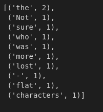
Let's create a function named tokens_top that takes in a text
as input and returns the top n most common tokens in a given text.

def tokens_top(text, n):
    # create tokens
    tokens = nltk.word_tokenize(text)

    # create the frequency distribution
    freqdist = nltk.FreqDist(tokens)

    # return the top n most common tokens
    return freqdist.most_common(n)

# Call the function 
tokens_top(df.text[1], 10)

Output

Document-Term Matrix

It is a matrix that represents the frequency of terms that occur in a collection of documents.
The rows represent the documents in the corpus and the columns represent the terms .
The cells of the matrix represents the frequency or weight of each term.

We can implement this with scikit-learn's CountVectorizer

Example

#import the package
from sklearn.feature_extraction.text import CountVectorizer

def create_dtm(series):
    # Create an instance/object of the class
    cv = CountVectorizer()

    # create a dtm from the series parameter
    dtm = cv.fit_transform(series)

    # convert the sparse array to a dense array
    dtm = dtm.todense()

    # get column names
    features = cv.get_feature_names_out()

    # create a dataframe
    dtm_df = pd.DataFrame(dtm, columns = features)

    # return the dataframe
    return dtm_df
# Call the function for df['text].head
create_dtm(df['text'].head())

Output

Data Cleaning

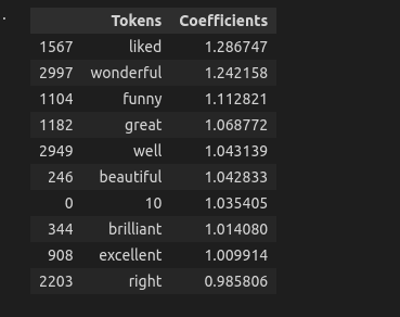
Feature Importance

Refers to the extent to which a specific feature/variable contributes to the
prediction or classification in sentiment analysis.

There are differet methods that can be used to determine feature importance:

• machine learning algorithms eg. decision trees and random forests
• statistical methods eg. correlation or regression analysis

feature importance is a useful tool in sentiment analysis as it can help identify
the most important features for accurately predicting the sentiment of a text.

Example
we'll define a function "top_n_tokens" that has 3 parameters
text, sentiment and n

the function will return the top n most important tokens
to predict the sentiment of the text.

We'll use LogisticRegression from sklearn.linear_model
with the following parameters:

• solver = 'lbfgs'
• max_iter = 2500

• random_state = 1234

  from sklearn.linear_model import LogisticRegression

  def top_n_tokens(text, sentiment, n):
  # create an instance of the class
  lgr = LogisticRegression(solver = 'lbfgs', max_iter = 2500, random_state = 1234)
  cv = CountVectorizer()

  # create the DTM
  dtm = cv.fit_transform(text)
  
  # fit the logistic regression model
  lgr.fit(dtm, sentiment)
  
  # get the coefficients
  coefs = lgr.coef_[0];
  
  # create the features/column names
  features = cv.get_features_names_out()
  
  # create the dataframe
  df = pd.DataFrame({'Tokens' : features, 'Coefficients' : coefs}) 
  # return the largest n
  return df.nlargest(n, coefficients)
  # Test if on df['text]
  top_n_tokens(df.text, df.label, 10)
  

Output

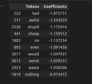
To validate the hypothesis that the most important features will be the ones that
indicate a strong positive sentiment, let's look at the 10 smallest coefficients.

from sklearn.linear_model import LosticRegression

def bottom_n_tokens(text, sentiment, n):
    # create an instance of the class
    lgr = LogisticRegression(solver = 'lbfgs', max_iter = 2500, random_state = 1234)
    cv = CountVectorizer()

    # create the DTM
    dtm = cv.fit_transform(text)

    # fit the logistic regression model
    lgr.fit(dtm, sentiment)

    # get the coefficients
    coefs = lgr.coef_[0];

    # create the features/column names
    features = cv.get_features_names_out()

    # create the dataframe
    df = pd.DataFrame({'Tokens' : features, 'Coefficients' : coefs})

    # return the smallest n
    return df.nmallest(n, coefficients)
# Test if on df['text]
bottom_n_tokens(df.text, df.label, 10)

Output

In the example that we've covered till this far we've used labelled data
What if we do not have labelled data?
Then we can use pre-trained models such as:

• TextBlob -VADER
• Stanford ColeNLP
• Google Cloud Natural Language API
• Hugging Face Transformers

Let's explore TextBlob

TextBlob

It is a Python library that provides a simple API for performing common
NLP tasks such as sentiment analysis.
It uses a pre-trained model to assign a sentiment score to a piece of text, ranging from -1 to 1

It is built on top of NLTK (natural language toolkit)
It also provides additional information such as:

• subjectivity score

It returns the sentiment of agiveen data in the format of a named tuple as follows:
(polarity, subjectivity)

polarity score is a float within the range of [-1.0, 1.0].

• it aims at differentiating whether the text is positive or negative

subjectivity is a float within the range [0.0, 1.0]

• 0.0 is very objective
• 1.0 is very subjective

TextBlob also provides other features such as:

• part-of-speech tagging
• a noun phrase extraction

Example

Let's define a function named polarity_subjectivity that accepts two argument.
The function uses TextBlob to the provided text
if print_results = True, prints polarity and subjectivity of the text elseM
returns a tuple of float values 1st being polarity and 2nd being subjectivity

You can install TextBlob using

!pip install textblob

#import TextBlob
from textblob import TextBlob

def polarity_subjectivity(text = sample, print_results = False):
    # create an instance of TextBlob
    tb= TextBlob(text)

    # if condition is metm print the results
    if print_results:
        print(f"Polarity is {round(tb.sentiment[0], 2)} : Subjectivity {round(tb.sentiment[1], 2)}")
    else:
        return (tb.sentiment[0], tb.sentiment[1])

# Test the function
polarity_subjectivity(sample, print_results =  True)

Output

The results indicate that our sample has a slight positive polarity and it's relatively subjective thought not by a high degree

Let's define a function token_count that accepts a string and using nltk's word_tokenizer,
returns an integer number of tokens in the given string

Then define another function series_tokens that accepts a Pandas Series as argument
and aplies the function
token_count to the given series.
Use the second function on the top 10 rows of our dataframe

# import libraries
from nltk import word_tokenize

# Define the first function that counts the number of tokens in a given string
def token_count(string):
    return (len(word_tokenize(string)))

# Define the second function that applies the           token_count funnction to a given Pandas series
def series_tokens(series):
    return series.apply(token_count)

# Apply the function to the top 10 rows of the data frame
series_tokens(df.text.head(10))

Output

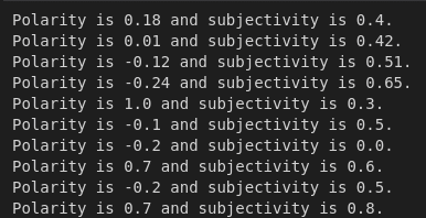
Let's define a function named series_polarity_subjectivity
that applies the polarity_subjectivity function we defined earlier

# define the function
def series_polarity_subjectivity(series):
    return series.apply(polarity_subjectivity)

# apply to the top 10 rows of df['text']
series_polarity_subjectivity(df['text'].head(10))

Output

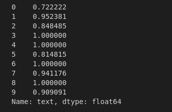
Measure of Complexity - Lexical Diversity

Lexical diversity refers to the variety of words used in a piece of writing or speech.
It is a measure of how often different words are used in a given text or speech and is often used as an indicator of the richnes and complexity of vocabulary.
It thus defines the number of unique tokens over the total number of tokens.

Example

Let's define a complexity function that accepts a string as an argument and returns the lexical complexity score defined as the number of unique tokens over the total number of tokens.

def complexity(string):
    # create a list of all tokens
    total_tokens = nltk.word_tokenize(string)

    # create a set of words(It keeps only unique values)
    unique_tokens = set(total_tokens)

    # Return the complexity measure
    if len(total_tokens) > 0:
        return len(unique_tokens) / len(total_tokens)

# apply the function to top 10 rows
df.text.head(10).apply(complexity)

Output

Some interesting insights the row at index 3 and 4 have the highest lexical diversity. All the tokens in them are totally unique.

Text Cleanup - Stopwords and Non-alphabeticals

This step ensures that the text data is in a constitent format and to remove noise,

irrelevant information and other inconsitencies.
Some of the techniques for text cleanup:

• Lowercasing
• Tokenization
• Stopword Removal
• Removing Punctuation
• Stemming and Lemmatization
• Removing URL's and mentions
• Removing emojis and emotions

Example

#import the library
from nltk.corpus imort stopwords

# Select only English stopwords
english_stop_words = stopwords.words('english')

# print the first 20
print(english_stop_words[:20])

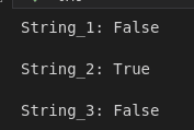
Let's look at an example to remove non-alphabetical
We'll use isalpha

string_1 = "Crite_Jes.cd"
string_2 = "a quick dog"
string_2 = "We are good!"

print(f"String_1: {string_1.isalpha()}\n")
print(f"String_1: {string_2.isalpha()}\n")
print(f"String_1: {string_3.isalpha()}\n")

Output

Comments

[Njeri Gitome]

Great details explained extensively!