Have you ever used the pen tool in Photoshop and tried to figure out how it works? Or perhaps wondered how SVGs get those perfect curves? Or have you ever seen those UI diagrams where the lines just know how to curve to attach to different boxes? These are splines. Splines are a mathematical way to produce curves and the cool part is they are infinitely accurate.
I originally wanted to cover Catmull-Rom, Bézier, and Basis Splines (B-Splines). Since I found that's a little too much for one post we'll start with Catmull-Rom.
Fun Fact: if you are like me you might have thought that "spline" is an acronym for somethings like "radar" or "scuba". It's actually a single word with a shared etymology to "splinter." It started as a thin piece of wood used in construction of things like boats. This evolved into a type bendy tool drafters used to draw curves: https://en.wikipedia.org/wiki/Flat_spline and finally was adopted for the computerized version of curve drawing.
Intuition
To really understand what's going on we need to look at graphing functions. If you've taken algebra and geometry you probably remember defining curves and shapes with functions. The simplest is a line, you might even know the form of a line function off the top of your head y = ax + b. Greater polynomials produce curves, where the greatest exponent is equal to the greatest number of times it can cross the x-axis or fold. For non-function shapes like circles that can have multiple y values per x value, you may have created parameterized equations or had to solve for a particular value like the equation for a circle: x^2 + y^2 = r^2. This is really what splines are under-the-hood but instead of representing them in terms of equations they are represented in terms of control points which makes them much easier to manipulate visually. Using varying amounts of control points and strategies (there are many types of splines with different behaviors) we can convert a set of points into an equation for a curve.
Catmull-Rom Spline

Honestly one of the better resources to understand Catmull-Rom splines is to watch two videos by Youtuber Javidx9 as he can do it better than I can:
https://www.youtube.com/watch?v=9_aJGUTePYo
I'll reiterate many of those points in this post.
In a Catmull-Rom spline we have 4-points. The two middle points indicate the start and the end points of the curve and the two end points are to help control the curvature. The overall intuition is that the curve is attracted to the the 2 anchor points and is repelled by the 2 control points. Or another way to think about it is that we're drawing the smoothest curve between two points but we need to more points to give us the initial direction and force that we leave the points at.
Let's start with the simplest 4-point case:
function catmullRomSpline(points, t) {
    const p0 = points[0];
    const p1 = points[1];
    const p2 = points[2];
    const p3 = points[3];

    const q0 = (-1 * t ** 3) + (2 * t ** 2) + (-1 * t);
    const q1 = (3 * t ** 3) + (-5 * t ** 2) + 2;
    const q2 = (-3 * t ** 3) + (4 * t ** 2) + t;
    const q3 = t ** 3 - t ** 2;

    return [
        0.5 * ((p0[0] * q0) + (p1[0] * q1) + (p2[0] * q2) + (p3[0] * q3)),
        0.5 * ((p0[1] * q0) + (p1[1] * q1) + (p2[1] * q2) + (p3[1] * q3)),
    ];
}
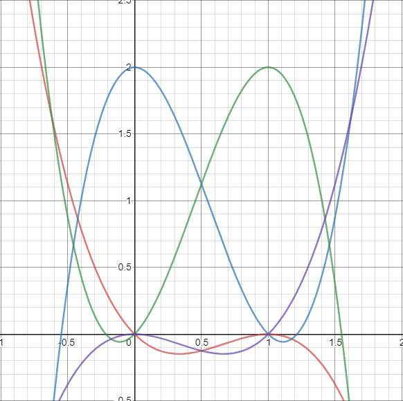
The formula is a specially chosen set of 4 cubic equations such that they intersect 2 and the x-axis at points 0 and 1, and the others have zeros at 0 and 1. Since these go from 2 to 0 though we need to scale them down by 0.5. The math is a bit beyond me but intuitively we can see there's a special property of these equations that makes this work even if it's a bit of black box.
Note that if you encounter these in the wild they'll probably be represented as matrices instead.
To draw the spline we simple call in a loop and take very small steps across t:
renderSpline() {
    const context = this.dom.canvas.getContext("2d");
    context.fillStyle = "#ff0000";
    for (const p of this.#points) {
        context.beginPath();
        context.arc(p[0], this.dom.canvas.height - p[1], 2, 0, 2 * Math.PI);
        context.fill();
    }
    context.fillStyle = "#0000ff";
    for (let i = 0; i < 1; i += 0.001) {
        const [x, y] = catmullRomSpline(this.#points, i);
        context.fillRect(x, this.dom.canvas.height - y, 1, 1);
    }
}
N-points

4 points is easy but we can continue the curve indefinitely. All we need to do is increment the indices by 1 and take the next 4 point window. Real points on the previous curves become control points on the next curve allowing us to make this continuous in segments.
The problem comes in when we're trying to figure out which segments we're between. The most naïve approach is to simply vary t from 0 to points.length - 3 instead of 0 to 1.
renderSpline() {
    const context = this.dom.canvas.getContext("2d");
    context.fillStyle = "#ff0000";
    for (const p of this.#points) { //draws points in red
        context.beginPath();
        context.arc(p[0], this.dom.canvas.height - p[1], 2, 0, 2 * Math.PI);
        context.fill();
    }
    context.fillStyle = "#0000ff";
    for (let i = 0; i < this.#points.length - 3; i += 0.001) {
        const [x, y] = catmullRomSpline(this.#points, i);
        context.fillRect(x, this.dom.canvas.height - y, 1, 1);
    }
}
We also need to change the spline function:
function catmullRomSpline(points, t) {
    const i = Math.floor(t);
    const p0 = points[i];
    const p1 = points[i + 1];
    const p2 = points[i + 2];
    const p3 = points[i + 3];

    const remainderT = t - Math.floor(t);

    const q0 = (-1 * remainderT ** 3) + (2 * remainderT ** 2) + (-1 * remainderT);
    const q1 = (3 * remainderT ** 3) + (-5 * remainderT ** 2) + 2;
    const q2 = (-3 * remainderT ** 3) + (4 * remainderT ** 2) + remainderT;
    const q3 = remainderT ** 3 - remainderT ** 2;

    return [
        0.5 * ((p0[0] * q0) + (p1[0] * q1) + (p2[0] * q2) + (p3[0] * q3)),
        0.5 * ((p0[1] * q0) + (p1[1] * q1) + (p2[1] * q2) + (p3[1] * q3)),
    ];
}
We take the floor to figure out which index should be the starting index for the value of t and then calculate where along the path we are based on the remainder.
This works for painting it but it's less useful for doing other things. What would be nice is if t was normalized from 0 to 1 with 1 being the ending point. We can't simply multiply this normalized t by points.length / 3 because the segments aren't the same length. If that doesn't make sense check the end of javidx9's video for one type of visual demonstration. What we really need is to figure out how long each segment is.
Estimation
There's no fancy math to measure a curve, just estimation. How do we estimate? Well, we can measure lines and if those lines are really small they get really close to recreating the actual curve.
However there's a little more here than just being able to normalize. Having approximations of complex functions can be very useful. Firstly, we can make things more efficient when drawing. Instead of trying to take little byte-sized chunks we can be smarter about dividing it into line segments and making the calculations easier while hopefully preserving the overall look. We can even be judicial about which method we use. For example, maybe I want the user to be able to scale the curve up. For this I can have a real-time preview using the approximation so that it animates smoothly and then use the more accurate model when they settle their adjustment by releasing the mouse.
The other use for this is that once we have it as a bunch of line segments it's much easier to find the edges. This can be used to do things like trimming the canvas of extra whitespace while making sure we don't accidentally clip a bulging curve.
So let's get to it:
function approximateCurve(curveFunction, max, delta){
    const points = [];
    for(let t = 0; t <= max; t += delta){
        points.push(curveFunction(t));
    }
    return points;
}
Simple. We have a function that generates points with a domain from 0 to max and we can pass in the delta. Note that you need less than or equal to max, otherwise if you land exactly on max you'll drop the last point. Also, I made a slight update to catmullRomSpline:
function catmullRomSpline(points, t) {
  if(points.length <= i + 3){ //out of bounds then clamp
    return points[points.length - 2];
  }

  //Omitted Stuff
}
The guard clause at the top prevent you from going out-of-bounds, instead you will be clamped to the final point. This is useful if the deltas don't perfectly fit.
Here's how I draw it:
context.strokeStyle = "#ff00ff";
context.lineWidth = 1;
context.beginPath();
const approximatePoints = approximateCurve(catmullRomSpline.bind(null, this.#points), this.#points.length - 3, 0.01);
context.moveTo(approximatePoints[0][0], this.dom.canvas.height - approximatePoints[0][1]);
for(let i = 1; i < approximatePoints.length; i++){
    context.lineTo(approximatePoints[i][0], this.dom.canvas.height - approximatePoints[i][1]);
}
context.stroke();
This is a trivial draw a series of lines routine. Note that I use context.beginPath to clear out any earlier stroking. The catmullRomSpline function specifically takes points as the first parameter for this reason. We can partially apply using bind so we have the curve in terms of t alone and we only draw the middle segments, not the end control points. And as always we need to convert out upwards growing y back into the proper row which grows down.
Here's delta = 0.5:

Here's delta = 0.01:
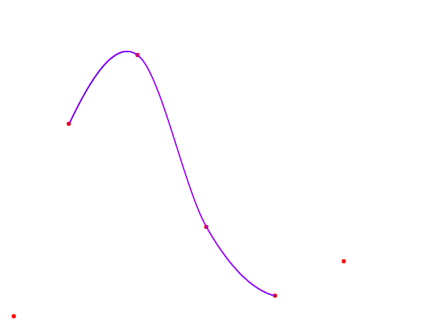
As we give higher deltas, we get a better approximation (magenta).
Measurement
Measurement isn't too hard. Now that we have the list of approximate points we just measure the lines between the points which is just Pythagoras's Theorem.
function measureSegments(segs){
    let length = 0;
    let lastPoint = segs[0];
    for(let i = 1; i < segs.length; i++){
        const currentPoint = segs[i];
        length += Math.sqrt((currentPoint[0] - lastPoint[0])**2 + (currentPoint[1] - lastPoint[1])**2);
        lastPoint = currentPoint;
    }
    return length;
}
And this gives us the total length of the curve.
You can also easily expand this to 3 dimensions (or even n-dimensions) by adding a more terms under the square root. In fact finding the length might be it's own function, I'll let you decide.
Just remember, this is an estimation and you're only as accurate as the number of line segments so if things feel a bit off you can play around to find the best trade off of speed and accuracy.
But actually the function above doesn't give us quite what we need for the normalization task even though it has it's own utility. We really need the length at each control point. So we'll update it to return a list of lengths, one for each point (the last element should have the same total distance).
function measureSegments(segs){
    const lengths = [0]; //first point is always at position 0
    let lastPoint = segs[0];
    for(let i = 1; i < segs.length; i++){
        const currentPoint = segs[i];
        lengths.push(Math.sqrt((currentPoint[0] - lastPoint[0])**2 + (currentPoint[1] - lastPoint[1])**2));
        lastPoint = currentPoint;
    }
    return lengths;
}
Normalization
Now that we have the lengths per control point we can finally move to creating a function that can produce the curve using a normalized t between 1 and 0. It's not hard but it's a little confusing so bear with me:
function normalizeCurve(curveFunc, max, delta){
    const segmentLengths = [0]; //first point is always position 0
    for(let i = 1; i <= max; i++){
        const approximatePoints = approximateCurve(curveFunc, i - 1, i, delta);
        const approximationSegmentLengths = measureSegments(approximatePoints);
        const length = approximationSegmentLengths.reduce((sum, l) => sum + l, 0);
        segmentLengths.push(length);
    }
    const maxLength = segmentLengths.reduce((sum, l) => sum + l, 0);

    return function(t){
        if(t < 0){
            return curveFunc(0);
        } else if (t > 1){
            return curveFunc(1);
        }

        const currentLength = t * maxLength;
        let totalSegmentLength = 0;
        let segmentIndex = 0;
        while(currentLength > totalSegmentLength + segmentLengths[segmentIndex + 1]){
            segmentIndex++;
            totalSegmentLength += segmentLengths[segmentIndex];
        }

        const segmentLength = segmentLengths[segmentIndex + 1];
        const remainderLength = currentLength - totalSegmentLength;
        const fractionalRemainder = remainderLength / segmentLength;
        return curveFunc(segmentIndex + fractionalRemainder);
    }
}
There's also a small update to approximateCurve to specify the min as well as the max so we can approximate a window of a function:
function approximateCurve(curveFunction, min, max, delta){
    const points = [];
    for(let t = min; t <= max; t += delta){
        points.push(curveFunction(t));
    }
    return points;
}
Ok, first off, like with the approximateCurve we're taking in the partially applied function but we'll also be returning a function. The function will be the curve function with a normalized t parameter. max is the max of the original function and delta is the size of microsegments used for approximation. I find the last parameter kinda odd to pass in as a user but it is necessary as you may want to tune the performance/accuracy tradeoff.
Here's where things get a little hard to mentally juggle because the terminology overlaps. We have two sets of "segments." We have the tiny microsegments that are used in the approximation, and we have the normal segments that span between the control points. What we're doing is estimating the length of each segment between the control points (segmentLengths) by adding up the lengths of the micro line segments (approximationSegmentLengths).
Once that's precalculated we can construct the new function. First we add guard clauses to clamp out-of-bounds values of t to the end. Then we multiply t by the maxLength (length of all segments added up) to get the distance along the curve of the point we're interested in. Then we start searching for the starting point. We check if the distance along the curve of the next point in the list is greater than our distance, if so then we've found the starting segment otherwise we keep incrementing. When we have the index of the starting segment, we subtract the total length up until that point from the distance we're looking for. This leave us with a remainder. We divide the remainder by the segment length to get the ratio of the length between these two points where the target falls. Finally we add the index of the starting point (remember the original function's domain was between 0 and points.length - 3) to the factionalRemainder to get the point in terms of the original function's t. Whew. I hope that's understandable.
Here's how I use it:
context.fillStyle = "#cc00ff";
const normalCurve = normalizeCurve(catmullRomSpline.bind(null, this.#points), this.#points.length - 3, 0.001);
for (let i = 0; i < 1; i += 0.001) {
    const [x, y] = normalCurve(i);
    context.fillRect(x, this.dom.canvas.height - y, 1, 1);
}
What did this buy us? Well for static visual examples not much but I might need this later. Maybe if you were animating the curve by drawing it would be helpful to get the speed right. It's a tool in the toolbox but if you can survive without it, it's a lot of extra calculation you can drop.
Slope and Normals
Nope, it's not the same thing as "normalization". A "normal" is a vector that is perpendicular to a surface. Imagine if the curve was a rollercoaster track, how should you draw that? Which way do the tops of people's heads point? Which way to the cars face? Slope and normals are useful for drawing things oriented along the spline, but they can also be highly useful for more advanced topics particularly in the 3D space.
You could approximate slope by taking tiny deltas along the curve and calculating their y/x but once you get infinitely small you just invented calculus, so we take the derivative of the spline equation with regards to t:
function catmullRomGradient(points, t){
    const i = Math.floor(t);
    const p0 = points[i];
    const p1 = points[i + 1];
    const p2 = points[i + 2];
    const p3 = points[i + 3];

    if (points.length <= i + 3) { //out of bounds then clamp
        return points[points.length - 2];
    }

    const remainderT = t - i;

    const q0 = (-3 * remainderT ** 2) + (4 * remainderT) -1;
    const q1 = (9 * remainderT ** 2) + (-10 * remainderT);
    const q2 = (-9 * remainderT ** 2) + (8 * remainderT) + 1;
    const q3 = (3 * remainderT ** 2) - (2 * remainderT);

    return [
        0.5 * ((p0[0] * q0) + (p1[0] * q1) + (p2[0] * q2) + (p3[0] * q3)),
        0.5 * ((p0[1] * q0) + (p1[1] * q1) + (p2[1] * q2) + (p3[1] * q3)),
    ];
}
Easy (as long as you remember your calc 1). This function gets us the slope at any point as [dx,dy]. The normal is defined as a vector that is perpendicular to the slope. To get that it's just -y/x which in vector form would be [-dy, dx] or [dy,-dx].
How to move points on a canvas
If you are building your own spline drawing functions it's likely you will want to know how to drag-and-drop the points because that's just what everyone does in these demos. We need 3 events:
function onPointerDown(){}
function onPointerUp(){}
function onPointerMove(){}
We'll only register the first though:
const canvas = document.querySelector("canvas");
canvas.addEventListener("pointerdown", onPointerDown);
This will check when we click or touch or tap down. Here we want to save some data, namely the point we clicked as well as the position when we started the drag:
let lastPointerX;
let lastPointerY;
let selectedIndex;
//points is your array of points
function onPointerDown(e){
const rect = canvas.getBoundingClientRect();
        lastPointerX = e.offsetX;
        lastPointerY = rect.height - e.offsetY;
        selectedIndex = points.findIndex(p => inRadius(lastPointerX, lastPointerY, 4, p[0], p[1]));

    if(selectedIndex > -1){
        selectedPointX = points[selectedIndex][0];
        selectedPointY = points[selectedIndex][1];
        canvas.addEventListener("pointermove", onPointerMove);
        canvas.addEventListener("pointerup", onPointerUp);
        canvas.removeEventListener("pointerdown", onPointerDown);
    }
}
Keep in mind y is still reversed so we need to change it. the event offsetX and offsetY are the x and y relative to the edge of the target, a handy shortcut so you don't need to calculate it yourself. To get the selected index we loop over the points and check if the point clicked close to it:
function inRadius(x,y,r, tx,ty){
    return Math.sqrt((x - tx)**2 + (y - ty)**2) <= r;
}
This is just checking the distance from the click to a point and if it's under a certain threshold then we consider it a match. You can play around with values that make sense, on a mobile device you might need a much larger radius than on a desktop with a mouse.
If we find a point (index not -1), then we capture it's current position and register two events for pointerup and pointermove. We also disable the current event as it's not necessary until we put the pointer back down.
onPointerMove(e){
    const rect = canvas.getBoundingClientRect();
    const currentPointerX = e.offsetX;
    const currentPointerY = rect.height - e.offsetY;
    currentOffsetX = currentPointerX - lastPointerX;
    currentOffsetY = lastPointerY - currentPointerY;

    const selectedPoint = points[selectedIndex];
    selectedPoint[0] = selectedPointX + currentOffsetX;
    selectedPoint[1] = selectedPointY - currentOffsetY;
    renderSpline();
}
Here we're getting the location of the pointer again and then figuring out how much we moved since we started the drag. We then add those values to the original value of the selected point. You could also get the delta between each move and add it to the current location of the selected point as well, however I like to do this instead because it gives me options on how to handle the interaction. If we implemented a move cancel event we'd want to revert to the original location. Or perhaps there is a mechanism to confirm the move since positioning things precisely can be tedious. At the end we render the spline so it shows up. Remember we could do optimizations here with approximation if the spline was really intense.
Finally:
onPointerUp(e){
    const selectedPoint = points[selectedIndex];
    selectedPoint[0] = selectedPointX + currentOffsetX;
    selectedPoint[1] = selectedPointY - currentOffsetY;
    renderSpline();
    canvas.removeEventListener("pointermove", onPointerMove);
    canvas.removeEventListener("pointerup", onPointerUp);
    canvas.addEventListener("pointerdown", onPointerDown);
}
We then do the same thing on pointerup. In this case it's not strictly necessary to set the point but it could be useful in a move cancel/confirm setup. Lastly, we unregister the move and up event as we don't need them until the pointer goes down again, and so we need to listen to that again.
That was quite lot of info, I hope I could make it understandable and useful. I would like continue to discuss other types of splines in future updates so look forward to it.

Top comments (0)