The Matrix Calculus You Need For Deep Learning (Notes from a paper by Terence Parr and Jeremy…

The Matrix Calculus You Need For Deep Learning (Notes from a paper by Terence Parr and Jeremy Howard)

Table of Contents

• Review: Scalar derivative rules
• Introduction to vector calculus and partial derivatives
• Matrix calculus
• Generalization of the Jacobian
• Derivatives of vector element-wise binary operators
• Vector sum reduction
• The Chain Rules
• Resources

Jeremy’s courses show how to become a world-class deep learning practitioner with only a minimal level of scalar calculus, thanks to leveraging the automatic differentiation built in to modern deep learning libraries. But if you really want to really understand what’s going on under the hood of these libraries, and grok academic papers discussing the latest advances in model training techniques, you’ll need to understand certain bits of the field of matrix calculus.

Review: Scalar derivative rules

Hopefully you remember some of these main scalar derivative rules. If your memory is a bit fuzzy on this, have a look at Khan academy video on scalar derivative rules.

Basic rules of derivatives

There are other rules for trigonometry, exponential, etc., which you can find at Khan Academy differential calculus course.

Introduction to vector calculus and partial derivatives

Neural network layers are not single functions of a single parameter, f(x). So, let’s move on to functions of multiple parameters such as f(x,y). For example, what is the derivative of xy (i.e., the multiplication of x and y)?

Well, it depends on whether we are changing x or y. We compute derivatives with respect to one variable (parameter) at a time, giving us two different partial derivatives for this two-parameter function (one for x and one for y). Instead of using operator d/dx, the partial derivative operator is ∂/ ∂x (a stylized d and not the Greek letter δ ). So ∂(xy)/ ∂x and ∂(xy)/ ∂y are the partial derivatives of xy; often, these are just called the partials.

The partial derivative with respect to x is just the usual scalar derivative, simply treating any other variable in the equation as a constant. Consider function f(x,y) = 3x²y. The partial derivative with respect to x is written ∂(3x²y*)/ ∂x.* There are three constants from the perspective of ∂/ ∂x : 3, 2, and y. Therefore, ∂(3x²y)/ ∂x = 3y∂(x²)/ ∂x = 3y(2x) = 6xy. The partial derivative with respect to y treats x like a constant and we get ∂(3x²y)/ ∂y = 3x². You can learn more on Khan Academy video on partials.

So from above example if f(x,y) = 3x²y, then

Gradient of f(x,y)

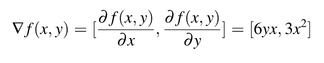
So the gradient of f(x,y) is simply a vector of its partial.

Matrix calculus

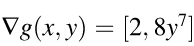
When we move from derivatives of one function to derivatives of many functions, we move from the world of vector calculus to matrix calculus. Let us bring one more function g(x,y) = 2x + y⁸. So gradient of g(x,y) is

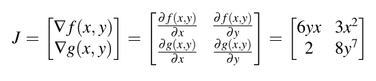
Gradient vectors organize all of the partial derivatives for a specific scalar function. If we have two functions, we can also organize their gradients into a matrix by stacking the gradients. When we do so, we get the Jacobian matrix (or just the Jacobian ) where the gradients are rows:

Numerator layout of Jacobian

Generalization of the Jacobian

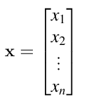
To define the Jacobian matrix more generally, let’s combine multiple parameters into a single vector argument: f(x,y,z) => f( x ). Lowercase letters in bold font such as x are vectors and those in italics font like x are scalars. xi is the ith element of vector x and is in italics because a single vector element is a scalar. We also have to define an orientation for vector x. We’ll assume that all vectors are vertical by default of size n X 1:

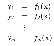
With multiple scalar-valued functions, we can combine them all into a vector just like we did with the parameters. Let y = f(x) be a vector of m scalar-valued functions that each take a vector x of length n= | x | where | x | is the cardinality (count) of elements in x. Each fi function within f returns a scalar just as in the previous section

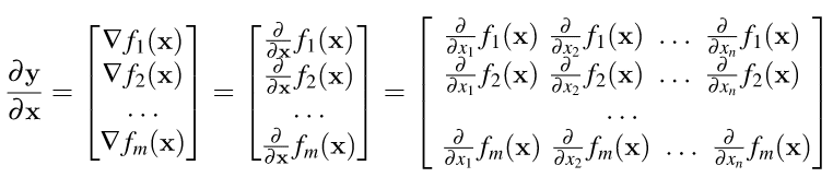
Generally speaking, though, the Jacobian matrix is the collection of all m X n possible partial derivatives (m rows and n columns), which is the stack of m gradients with respect to x :

Derivatives of vector element-wise binary operators

By “element-wise binary operations” we simply mean applying an operator to the first item of each vector to get the first item of the output, then to the second items of the inputs for the second item of the output, and so forth.We can generalize the element-wise binary operations with notation y= f(w) O g(x) where m = n = | y | = | w | = | x |. The O symbol represents any element-wise operator (such as +) and not the o function composition operator.

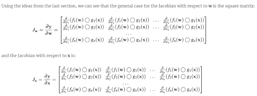
That’s quite a furball, but fortunately the Jacobian is very often a diagonal matrix, a matrix that is zero everywhere but the diagonal.

Vector sum reduction

Summing up the elements of a vector is an important operation in deep learning, such as the network loss function, but we can also use it as a way to simplify computing the derivative of vector dot product and other operations that reduce vectors to scalars.

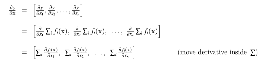
Let y=sum(f(x)) = Σ fi ( x ). Notice we were careful here to leave the parameter as a vector x because each function fi could use all values in the vector, not just xi. The sum is over the results of the function and not the parameter. The gradient ( 1 X n Jacobian) of vector summation is:

The Chain Rules

We can’t compute partial derivatives of very complicated functions using just the basic matrix calculus rules. Part of our goal here is to clearly define and name three different chain rules and indicate in which situation they are appropriate.

The chain rule is conceptually a divide and conquer strategy (like Quicksort) that breaks complicated expressions into sub-expressions whose derivatives are easier to compute. Its power derives from the fact that we can process each simple sub-expression in isolation yet still combine the intermediate results to get the correct overall result.

The chain rule comes into play when we need the derivative of an expression composed of nested subexpressions. For example, we need the chain rule when confronted with expressions like d(sin(x²))/dx.

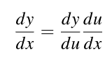
• Single-variable chain rule ** :-** Chain rules are typically defined in terms of nested functions, such as y = f(u) where u= g(x) so y= f(g(x)) for single-variable chain rules.

Formulation of the single-variable chain rule

To deploy the single-variable chain rule, follow these steps:

1. Introduce intermediate variables for nested sub-expressions and sub-expressions for both binary and unary operators; example, X is binary, sin (x) and other trigonometric functions are usually unary because there is a single operand. This step normalizes all equations to single operators or function applications.
2. Compute derivatives of the intermediate variables with respect to their parameters.
3. Combine all derivatives of intermediate variables by multiplying them together to get the overall result.
4. Substitute intermediate variables back in if any are referenced in the derivative equation.

• Single-variable total-derivative chain rule :- The total derivative assumes all variables are potentially codependent whereas the partial derivative assumes all variables but x are constants.

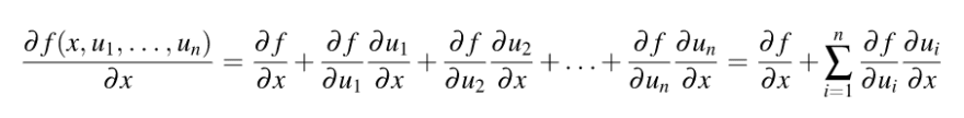
This chain rule that takes into consideration the total derivative degenerates to the single-variable chain rule when all intermediate variables are functions of a single variable.

A word of caution about terminology on the web. Unfortunately, the chain rule given in this section, based upon the total derivative, is universally called “multivariable chain rule” in calculus discussions, which is highly misleading! Only the intermediate variables are multivariate functions.

• Vector chain rule :- Vector chain rule for vectors of functions and a single parameter mirrors the single-variable chain rule.

If y= f(g(x)) and x is a vector . The derivative of vector y with respect to scalar x is a vertical vector with elements computed using the single-variable total-derivative chain rule.

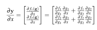
The goal is to convert the above vector of scalar operations to a vector operation. So the above RHS matrix can also be implemented as a product of vector multiplication.

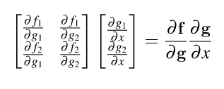
That means that the Jacobian is the multiplication of two other Jacobians. To make this formula work for multiple parameters or vector x , we just have to change x to vector x in the equation. The effect is that ∂g/ ∂x and the resulting Jacobian, *∂f/ ∂x * , are now matrices instead of vertical vectors. Our complete vector chain rule is:

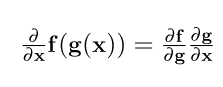
Please note here that matrix multiply does not commute, the order of (**∂f/ ∂x)(∂g/ ∂x) **matters.

For completeness, here are the two Jacobian components :-

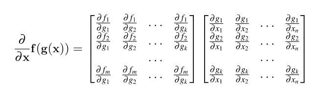
where m = | f |, n = | x | and k = | g |. The resulting Jacobian is m X n. (an m X k matrix multiplied by a k X _n _ matrix).

We can simplify further because, for many applications, the Jacobians are square ( m = n ) and the off-diagonal entries are zero.

Resources

1.The original paper.

1. There are some online tools which can differentiate a matrix for you:

• Wolfram Alpha
• Matrix calculus Differentiator.

1. More matrix calculus.