
Introduction
Gradient descent is one of the most popular optimization algorithms in machine learning and deep learning,
it used to find the local minimum of a differentiable function.
In machine learning, gradient descent is used to find the values of parameters that minimize the cost function (loss function).
“A gradient measures how much the output of a function changes if you change the inputs a little bit.” — Lex Fridman
In this article, we’ll go through
What is gradient in the first place ?!
hypothesis function(st-line equation).
Cost function for linear regression.
Gradient descent for linear regression.
What is a gradient in the first place ?!
In mathematics, a gradient is another name for the slope of the st-line or how steep is the st-line.

Gradient = slope = derivative of a function
Hypothesis function and plotting different values of theta.
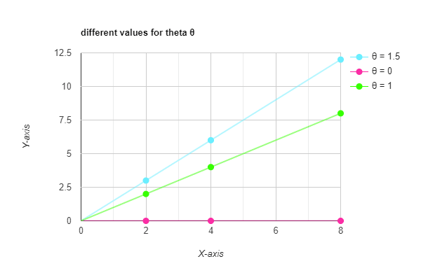
let’s start by taking an example,
we have 3 sample points ( 2, 2 ), ( 4, 4 ), ( 8, 8 )

the straight-line equation (Hypothesis function)

it’s also written as: h(x)= y = θ1 + θ2 x
let’s make it simple enough and make θ1= 0.
the equation will be:
h (x) = θ2.X
now we want to draw a straight line h(x) = θ2 x to best fit the data
then predict (y) values of training data (x,y) to see how good the line fits the data by calculating the cost function ( loss function )
of course in this example, it's obvious that we want to choose θ2= 1 to best fit the line but with too many samples ( thousands or millions ) it’s not that easy
we have to use Gradient descent or other algorithms to choose the best parameters,
even if this is a very simple example but it will clear the vision about how the parameters are chosen and how gradient descent works.
I’m choosing two values for θ2 ( 1.5 and 0 )
( that’s the Gradient descent rule to choose the best parameters but we are choosing different values to understand how it goes)
so now the blue line equation will be h(x) = 1.5 x
and the red line equation h (x) = 0x = 0
so the slope = tan ( θ ) = tan( 0 ) = zero degree.
that will make the line lie on the x-axis as you see

and the last line we will draw of course will be with θ = 1
the green st-line equation will be
h(x) = x
and that will make the line pass through each point of the samples. (which is not good by the way and called overfitting but in this case let’s assume it's a good thing)
Cost function and Plotting different values for theta.
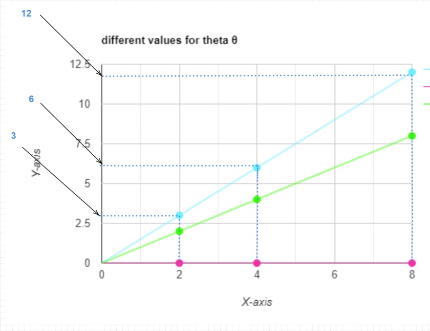
Now we have three models to choose from the best model which makes the best predictions.
h(x) = 1.5 x
h(x) = 0
h(x) = x
We want each equation of those to make predictions of output h(x) based on a given value of the input (x) by using our training examples
Then we calculate the cost function ( model accuracy ) to choose the best model of them.
We have 3 training examples of (x,y)
(2,2 ), (4,4),(8,8)
we’ll start by:
h(x) = 1.5x
for x = 2 , h(x)=1.5*2 = 3
for x = 4 , h(x)=1.5*4 = 6
for x = 8, h(x)=1.5*8 = 12
It’s time to calculate the cost function (model accuracy)
The cost function for linear regression.

where
θ: equation parameters
i: index
m: number of training examples( in our case we have 3 training examples)
h(x): predicted value
y: expected value
we’ll calculate J(1.5 ) , J(0) , J(1)
let’s substitute our predicted values of h(x)
for J(1.5)
h(2) = 3, h(4)= 6 and h(8)= 12
so, J(1.5) = 1/2m ( (3–2 )² +(6–4)² +(12–8 )²)
J(1.5) = 1/2*3 ( 1² + 2² + 4²) = 1/6 ( 21)
J(1.5) = 3.5
We will do the same for J(0)
h(x) = 0 so, all outputs will be equal 0
the cost will be as follow
J(0) = 1/2m ( (0–2 )² +(0–4)² +(0–8 )²)
J(0) = 1/6* (84) = 14
the last cost will be for θ = 1
**h(x) = x
h(2) = 2 , h(4)= 4 and h(8)= 8
J(1) = 1/2m ( (2–2 )² +(4–4)² +(8–8 )²)
J(1) = 1/6 ( 0 )
J(1) = Zero**
which means that h(1) make perfect predictions
So, we’ll choose θ= 1 for the best predictions,
what we just did in the previous steps is what the Gradient descent algorithm does.
Gradient Descent For Linear Regression (How it works).
Now we want to see the relationship between J(θ) and θ
we have 3 points to plot ( θ, J(θ) ) with J(θ) on the y-axis and θ on the x-axis
Points : (0, 14) , (1, 0) and (1.5, 3.5)

the perfect choice of parameters will make J(θ) = zero.
but, a perfect model with 100% accuracy working with a lot of data is rare if not impossible at least for now.
gradient descent algorithm starts by initializing starting point (x,y)
and then tries to find the Global minimum ( the value of θ gives minimum value to J(θ))
which in our graph the point ( 1, 0 )(Global minimum)
when θ=1, J(θ) = 0.
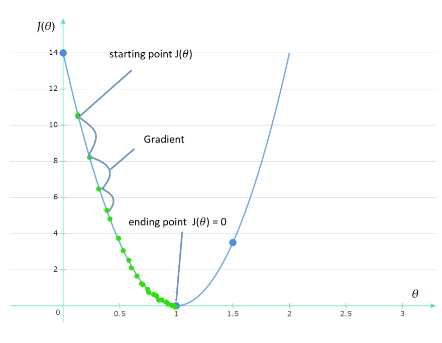
But how the heck the gradient descent algorithm does that ?!
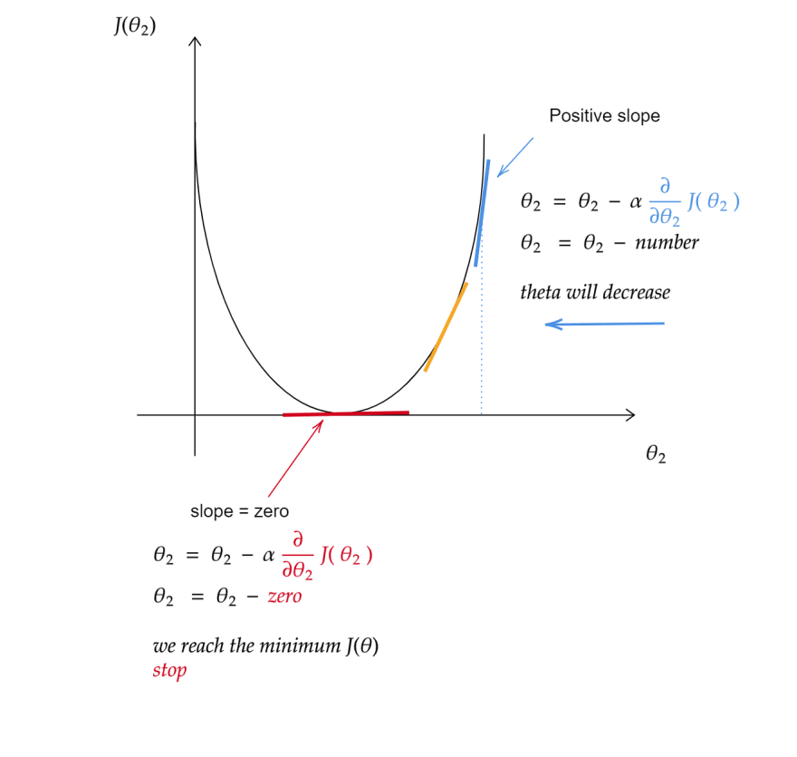
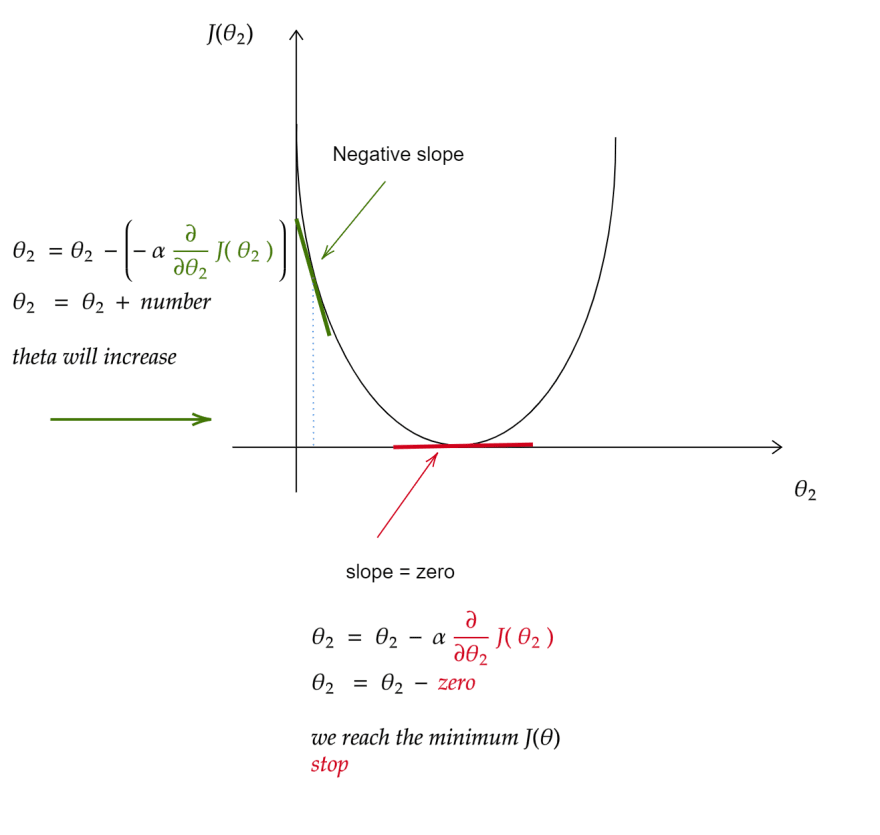
Now it’s time to see the gradient descent general formula

Where
θ : parameter ( also called weight )
j = 1 or j = 2 ( number of parameters θ)
α : learning rate
∂ / ∂θ : partial derivative ( slope of straight line )
J(θ1,θ2) : cost function
In our example θ1 = 0, so we just have θ2 to deal with
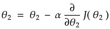
gradient descent algorithm goal is to find values for equation parameters (θ2) which make J(θ2) is minimum
it starts with an initial value of θ then update this value until converge ( reach the minimum cost )
θ2 ( new value ) = θ2 (initial value ) - α( number )* ∂/∂θ2 ( slope of the st- line )
gradient descent may do this step thousands of times or more with one or more parameters.
now let’s see how the slope of the straight line work in this equation
how it converges if the slope is positive
how it converges if the slope is negative

Top comments (0)