Recreate the Tesla Cybertruck in Matplotlib — Solution to Dunder Data Challenge #6
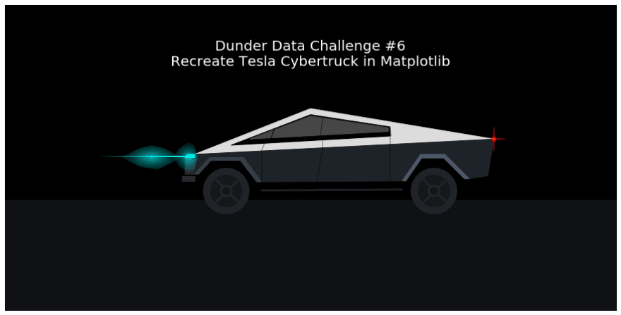
In this challenge, you will recreate the new Tesla Cybertruck unveiled last week using matplotlib. Our goal is to recreate this image below.

Begin Mastering Data Science Now for Free!
Take my free Intro to Pandas course to begin your journey mastering data analysis with Python.
Solution
Click the video below to view the animation and final solution.
Tutorial
A tutorial will now follow that describes the recreation. It will discuss the following:
- Figure and Axes setup
- Adding shapes
- Color gradients
- Animation
Understanding these topics should give you enough to start animating your own figures in matplotlib.
Figure and Axes setup
We first create a matplotlib Figure and Axes, remove the axis labels and tick marks, and set the x and y axis limits. The fill_between method is used to set two different background colors.
import numpy as np
import matplotlib.pyplot as plt
%matplotlib inline
fig, ax = plt.subplots(figsize=(16, 8))
ax.axis('off')
ax.set\_ylim(0, 1)
ax.set\_xlim(0, 2)
ax.fill\_between(x=[0, 2], y1=.36, y2=1, color='black')
ax.fill\_between(x=[0, 2], y1=0, y2=.36, color='#101115');

Shapes in matplotlib
Most of the Cybertruck is composed of shapes (patches in matplotlib terminology) — circles, rectangles, and polygons. These shapes are available in the patches matplotlib module. After importing, we instantiate single instances of these patches and then call the add_patch method to add the patch to the Axes.
For the Cybertruck, I used three patches, Polygon, Rectangle, and Circle. They each have different parameters available in their constructor. I first constructed the body of the car as four polygons. Two other polygons were used for the rims. Each polygon is provided a list of x, y coordinates where the corners are located. Matplotlib connects all the points in order and fills it in with the provided color.
from matplotlib.patches import Polygon, Rectangle, Circle
top = Polygon([[.62, .51], [1, .66], [1.6, .56]], color='#DCDCDC')
windows = Polygon([[.74, .54], [1, .64], [1.26, .6], [1.262, .57]],
                   color='black')
windows\_bottom = Polygon([[.8, .56], [1, .635], [1.255, .597],
                          [1.255, .585]], color='#474747')
base = Polygon([[.62, .51], [.62, .445], [.67, .5], [.78, .5],
                [.84, .42], [1.3, .423],[1.36, .51], [1.44, .51],
                [1.52, .43], [1.58, .44], [1.6, .56]],
                color="#1E2329")
left\_rim = Polygon([[.62, .445], [.67, .5], [.78, .5], [.84, .42],
                    [.824, .42], [.77, .49],[.674, .49],
                    [.633, .445]], color='#373E48')
right\_rim = Polygon([[1.3, .423], [1.36, .51], [1.44, .51],
                     [1.52, .43], [1.504, .43], [1.436, .498],
                     [1.364, .498], [1.312, .423]], color='#4D586A')

ax.add\_patch(top)
ax.add\_patch(windows)
ax.add\_patch(windows\_bottom)
ax.add\_patch(base)
ax.add\_patch(left\_rim)
ax.add\_patch(right\_rim)
fig

Learn more
I have free courses to get started learning data analysis using Python at Dunder Data. I am the author of the following books:
Tires
I used three Circle patches for each of the tires. You must provide the center and radius.
left\_tire = Circle((.724, .39), radius=.075, color="#202328")
right\_tire = Circle((1.404, .39), radius=.075, color="#202328")
left\_inner\_tire = Circle((.724, .39), radius=.052, color="#15191C")
right\_inner\_tire = Circle((1.404, .39), radius=.052,
                          color="#15191C")
left\_spoke = Circle((.724, .39), radius=.019, color="#202328")
right\_spoke = Circle((1.404, .39), radius=.019, color="#202328")
left\_inner\_spoke = Circle((.724, .39), radius=.011, color="#131418")
right\_inner\_spoke = Circle((1.404, .39), radius=.011, color="#131418")

ax.add\_patch(left\_tire)
ax.add\_patch(right\_tire)
ax.add\_patch(left\_inner\_tire)
ax.add\_patch(right\_inner\_tire)
ax.add\_patch(left\_spoke)
ax.add\_patch(right\_spoke)
ax.add\_patch(left\_inner\_spoke)
ax.add\_patch(right\_inner\_spoke)
fig

Axels
I used the Rectangle patch to represent the two 'axels' (this isn't the correct term, but you'll see what I mean) going through the tires. You must provide a coordinate for the lower left corner and a width and a height. You can also provide it an angle (in degrees) to further control its position. Notice that they are currently displayed over the inner tire circle. This will get fixed when we combine all the patches together.
left\_left\_axel = Rectangle((.687, .427), width=.104, height=.005,
                           angle=315, color='#202328')
left\_right\_axel = Rectangle((.761, .427), width=.104, height=.005,
                            angle=225, color='#202328')
right\_left\_axel = Rectangle((1.367, .427), width=.104, height=.005,
                            angle=315, color='#202328')
right\_right\_axel = Rectangle((1.441, .427), width=.104, height=.005,
                             angle=225, color='#202328')
ax.add\_patch(left\_left\_axel)
ax.add\_patch(left\_right\_axel)
ax.add\_patch(right\_left\_axel)
ax.add\_patch(right\_right\_axel)
fig

Other details
The front bumper, head light, tail light, door and window lines are added below. I used regular matplotlib lines for some of these. Those lines are not patches and get added to the Axes without any other additional method.
# other details
front = Polygon([[.62, .51], [.597, .51], [.589, .5], [.589, .445],
                 [.62, .445]], color='#26272d')
front\_bottom = Polygon([[.62, .438], [.58, .438], [.58, .423], [.62,
                         .423]], color='#26272d')
head\_light = Polygon([[.62, .51], [.597, .51], [.589, .5], [.589,
                      .5], [.62, .5]], color='aqua')
step = Polygon([[.84, .39], [.84, .394], [1.3, .397], [1.3, .393]],
                color='#1E2329')
# doors
ax.plot([.84, .84], [.42, .523], color='black', lw=.5)
ax.plot([1.02, 1.04], [.42, .53], color='black', lw=.5)
ax.plot([1.26, 1.26], [.42, .54], color='black', lw=.5)

ax.plot([.84, .85], [.523, .547], color='black', lw=.5)
ax.plot([1.04, 1.04], [.53, .557], color='black', lw=.5)
ax.plot([1.26, 1.26], [.54, .57], color='black', lw=.5)

# window lines
ax.plot([.87, .88], [.56, .59], color='black', lw=1)
ax.plot([1.03, 1.04], [.56, .63], color='black', lw=.5)

# tail light
tail\_light = Circle((1.6, .56), radius=.007, color='red', alpha=.6)
tail\_light\_center = Circle((1.6, .56), radius=.003, color='yellow',
                           alpha=.6)
tail\_light\_up = Polygon([[1.597, .56], [1.6, .6], [1.603, .56]],
                         color='red', alpha=.4)
tail\_light\_right = Polygon([[1.6, .563], [1.64, .56], [1.6, .557]],
                            color='red', alpha=.4)
tail\_light\_down = Polygon([[1.597, .56], [1.6, .52], [1.603, .56]],
                           color='red', alpha=.4)

ax.add\_patch(front)
ax.add\_patch(front\_bottom)
ax.add\_patch(head\_light)
ax.add\_patch(step)
ax.add\_patch(tail\_light)
ax.add\_patch(tail\_light\_center)
ax.add\_patch(tail\_light\_up)
ax.add\_patch(tail\_light\_right)
ax.add\_patch(tail\_light\_down)
fig

Color gradients for the head light beam
The head light beam has a distinct color gradient that dissipates into the night sky. This is a challenging to do. I found an excellent answer on Stack Overflow from user Joe Kington on how to do this. We begin, by using the imshow function which creates images from 3-dimensional arrays. We create a 100 x 100 x 4 array that represents 100 x 100 points of RGBA (red, green, blue, alpha) values. Every point has the same red, green, and blue values of (0, 1, 1) which represents the color alpha, but has an alpha value that ranges from 0 to 1. The further from the head light, the smaller the alpha. The alpha represents opacity. This slowly decreases the opacity until it reaches 0. The extent parameter controls the rectangular region (xmin, xmax, ymin, ymax) where the image will be shown.
import matplotlib.colors as mcolors
z = np.empty((100, 100, 4), dtype=float)
rgb = mcolors.colorConverter.to\_rgb('aqua')
z[:, :, :3] = rgb
alphas = np.linspace(0, 1, 100)[:, None]
alphas = np.tile(alphas, 100).T
z[:, :, -1] = alphas

im = ax.imshow(z, extent=[.3, .589, .501, .505], zorder=1)
fig

Proportional alphas
Below, two more aqua images are added. The alpha values are directly proportional to the distance from the center of the rectangular region defined by extent. They eventually decrease to 0.
# beam clouds
x = np.arange(100)
y = (50 - x) \*\* 2
z2 = np.empty((100, 100, 4), dtype=float)
rgb = mcolors.colorConverter.to\_rgb('aqua')
z2[:,:,:3] = rgb
z2[:, :, -1] = 1 - np.sqrt(y.reshape(1, -1) + y.reshape(-1, 1)) / 71
z2[:, :, -1] \*\*= 2
z2[:, :, -1] \*= .7

im2 = ax.imshow(z2, extent=[.55, .65, .45, .55], zorder=1)
im3 = ax.imshow(z2, extent=[.38, .58, .45, .55], zorder=1)
fig

Gradients in patches
Color gradients within patches is a bit more work. You’ll need to first create an image like we did above. Construct the patch setting the color to ‘none’ and add the patch as normal. Finally, call the set_clip_path method of the image passing it the patch.
beam\_cloud\_1 = Polygon([[.6, .45], [.57, .47], [.55, .5],
                        [.57, .53], [.6, .55], [.62, .54],
                        [.625, .52], [.63, .5], [.625, .48],
                        [.62, .46] ], color='none')

beam\_cloud\_2 = Polygon([[.58, .5], [.52, .53], [.48, .54],
                        [.44, .53], [.38, .5], [.44, .47],
                        [.5, .46], [.52, .47]], color='none')

ax.add\_patch(beam\_cloud\_1)
im2.set\_clip\_path(beam\_cloud\_1)

ax.add\_patch(beam\_cloud\_2)
im3.set\_clip\_path(beam\_cloud\_2)
fig

Creating a Function to Draw the Car
All of our work from above can be placed in a function that draws the car. This will be used when initializing our animation. The function is not shown, but just puts all of the above code in a single code block.
Animation
Animation in matplotlib is fairly straightforward. You must create a function that updates the position of the objects in your figure for every frame. This function is called repeatedly for each frame that you create.
In the update function below, we loop through each patch, line and image in our Axes and reduce the x-value of each plotted object by .015. This has the effect of moving the truck to the left. The trickiest part was changing the x and y values for the rectangular tire ‘axels’. Some basic trigonemtry helps calculate this.
Finally, the FuncAnimation class from the animation module is used to construct the animation. We provide it our update function and a function to call once to initialize the figure along with the number of frames and any extra arguments used during update.
def update(frame\_number, x\_delta, radius, angle):
    if frame\_number == 0:
        return
    ax = fig.axes[0]
    for patch in ax.patches:
        if isinstance(patch, Polygon):
            arr = patch.get\_xy()
            arr[:, 0] -= x\_delta
        elif isinstance(patch, Circle):
            x, y = patch.get\_center()
            patch.set\_center((x - x\_delta, y))
        elif isinstance(patch, Rectangle):
            xd\_old = -np.cos(np.pi \* patch.angle / 180) \* radius
            yd\_old = -np.sin(np.pi \* patch.angle / 180) \* radius
            patch.angle += angle
            xd = -np.cos(np.pi \* patch.angle / 180) \* radius
            yd = -np.sin(np.pi \* patch.angle / 180) \* radius
            x = patch.get\_x()
            y = patch.get\_y()
            x\_new = x - x\_delta + xd - xd\_old
            y\_new = y + yd - yd\_old
            patch.set\_x(x\_new)
            patch.set\_y(y\_new)

    for line in ax.lines:
        xdata = line.get\_xdata()
        line.set\_xdata(xdata - x\_delta)

    for image in ax.images:
        extent = image.get\_extent()
        extent[0] -= x\_delta
        extent[1] -= x\_delta

animation = FuncAnimation(fig, update, init\_func=draw\_car,
                          frames=110, repeat=False,
                          fargs=(.015, .052, 4))
Save animation
Finally, we can save the animation as an mp4 file (assuming you have ffmpeg). The html video tag is used in the markdown to display the animation.
animation.save('../images/tesla\_animate.mp4', fps=30, bitrate=3000)
Animation on YouTube
Here is the final animation on YouTube
Master Python, Data Science and Machine Learning
Immerse yourself in my comprehensive path for mastering data science and machine learning with Python. Purchase the All Access Pass to get lifetime access to all current and future courses . Some of the courses it contains:
- Exercise Python — A comprehensive introduction to Python (200+ pages, 100+ exercises)
- Master Data Analysis with Python — The most comprehensive course available to learn pandas. (600+ pages and 300+ exercises)
- Master Machine Learning with Python — A deep dive into doing machine learning with scikit-learn constantly updated to showcase the latest and greatest tools. (300+ pages)

Top comments (0)