The Trials And Tribulations Of The Traveling Salesman

The trials and tribulations of the traveling salesman!

As we dive deeper and deeper into the world of computer science, one thing starts to become very clear, very quickly: some problems seem to show up again and again, in the strangest of forms. In fact, some of the most famous problems in the history of computer science have no specific origin that anyone knows of. Instead, the same problem shows up in different forms and avatars, in different places around the world, at different time periods.

The hardest problems in software are the most fun to solve – and some of them haven’t even been figured out yet! One of these hard problems is the traveling salesman problem, and depending on whom you ask, it might be the most notorious of them all.

I first heard about the traveling salesman problem a few years ago, and it seemed super daunting to me at the time. To be totally honest, even coming back to it now, it still feels a little bit daunting, and it might seem scary to you, too. But something is different this time around: we’ve got a whole wealth of knowledge and context to draw from! Throughout this series, we’ve been building upon our foundation core of computer science, and returning to some of the same concepts repeatedly in an effort to understand them on a more technical level – but only when we feel fully equipped to do so. The same goes for this look into the the traveling salesman problem.

In order to understand why this problem is so notorious, we need to wrap our heads around what it is, how we can solve it, why it is important, and what makes it so hard. It might sound overwhelming, but we’ll get through it together, one step at a time.

So, let’s hop to it!

Geometry, circuits, and a dude named Hamilton

The idea behind the traveling salesman problem (TSP) is rooted in a rather realistic problem that many people have probably actually encountered. The thesis is simple: a salesman has to travel to every single city in an area, visiting each city only once. Additionally, he needs to end up in the same city where he starts his journey from.

The traveling salesman seeks to visit each city once, and end up in the same place he started.

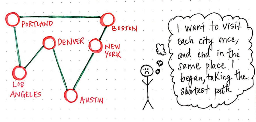
The actual “problem” within the traveling salesman problem is finding the most efficient route for the salesman to take. There are obviously many different routes to choose from, but finding the best one – the one that will require the least cost or distance of our salesman – is what we’re solving for.

In more ways than one, the practical aspects of this problem are reminscient of The Seven Bridges of Königsberg, a mathematical problem that we’re already familiar with, which was the basis for Euler’s invention of the field called “the geometry of position”, which we now know today as graph theory.

William Rowan Hamilton, Wikimedia Commons

But graph theory didn’t end with Euler and the city of Königsberg! Indeed, the Seven Bridge problem was just the beginning, and the traveling salesman problem is a prime example of someone building upon the ideas of those who came before him.

The “someone” in this scenario is none other than William Rowan Hamilton, an Irish physicist and mathematician who was inspired by and subsequently continued the research of mathematicians who came before him in order to create a subset of mathematical problems that are directly tied to the traveling salesman problem that we are familiar with today.

Comparing Eulerian and Hamiltonian paths.

In the late 1800’s, both Hamilton and the British mathematician Thomas Kirkman were working on mathematical problems that were fundamentally similar to TSP. Hamilton’s claim to fame was his work on deriving a something called a Hamiltonian path , which bears resemblance to Euler’s famous Eulerian path.

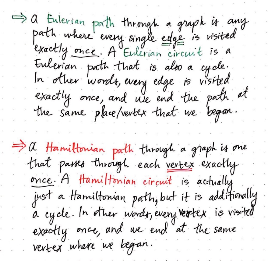
While a Eulerian path is a path where every single edge in a graph is visited once, a Hamiltonian path is one where every single vertex is visited exactly once.

By the same token, a Eulerian circuit is a Eulerian path that ends at the same vertex where it began, touching each edge once. A Hamiltonian circuit , on the other hand, is a Hamiltonian path that ends at the same vertex where it began, and touches each vertex exactly once.

TSP as a Hamiltonian circuit problem.

A good rule of thumb to determine whether a path through a graph is Hamiltonian or Eulerian is this:

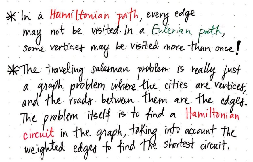
in a Hamiltonian path , every edge doesn’t need to be visited, but every node must visited – but only once! In comparison, in an Eulerian path, some vertices could be visited multiple times, but every edge can only ever be visited once.

The reason that Hamilton’s work, which is built upon Euler’s formulations, comes up in the context of the famous traveling salesman problem is that the job of the salesman – traveling to each city exactly once and ending up where he began – is really nothing more than a graph problem!

The icosian game, invented by W.R. Hamilton in the 1800's.

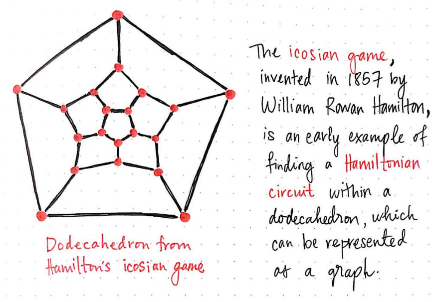
Hamilton’s work expanded graph theory to the point where he was actually solving the TSP before it was really a thing. Hamilton invented a game that was similar to the traveling salesman problem, which he called the icosian game , whose objective was to find a path through the points of a dodecahedron, or a polygon with 12 flat faces.

Hamilton’s game was eventually turned into an actual board game. And, if we think about it, even the icosian game is really just another variation on the traveling salesman problem! Just as as dodecahedron has 20 vertices, we could imagine Hamilton’s game as a map of 20 cities. Using this analogy, our traveling salesman would need to find a way through 20 cities, visiting each city once, and ending up exactly where he started.

Hamilton’s icosian game, © Puzzle Museum

Thus, the traveling salesman problem can really just be reformulated to be represented as a graph. Luckily, we have covered a whole lot of different topics when it comes to complex graphs. We’ve got a solid foundation to build upon, just like Hamilton did!

Once we’re able to wrap our heads around the fact that the traveling salesman problem is really just a graph traversal problem, we can start getting down to business. In other words, we can start trying to solve this problem. For our purposes, we won’t worry ourselves with trying to get the best solution or using the most efficient approach. Instead, we’ll start by simply trying to get some kind of solution to begin with. Using the old adage attributed to Kent Beck, we must first “Make it work” before we can even begin to think about making it “right” or “fast”.

So, let’s get to work and get our salesman on the road!

Brute-force to begin with

The traveling salesman in our example problem has it pretty lucky – he only has to travel between four cities. For simplicity’s sake, we’ll call these four cities w, x, y, and z. Because we know that TSP is a graph problem, we can visualize our salesman’s possible routes in the form of a weighted, undirected graph. We’ll recall that a weighted graph is one whose edges have a cost or distance associated with them, and an undirected graph is one whose edges have a bidirectional flow.

Looking at an illustrated example of our salesman’s graph, we’ll see that some routes have a greater distance or cost than others. We’ll also notice that our salesman can travel between any two vertices easily.

How can we solve for the optimal path starting and ending at node w?

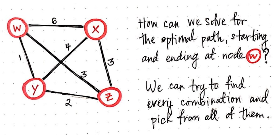
Let’s say that our salesman lives in city w, so that’s where he’ll start his journey from. Since we’re looking for a Hamiltonian cycle/circuit, we know that this is also where he will need to end up at the end of his adventures. So, how can we solve for the optimal path so that our salesman starts and ends at city (node) w, but also visits every single city (x, y, and z) in the process?

Remember, we’re not going to think about the most efficient strategy – just one that works. Since we’re going to use the brute-force approach, let’s think about what we’re really trying to solve for here. The brute-force approach effectively means that we’ll solve our problem by figuring out every single possiblity and then picking the best one from the lot. In other words, we want to find every single permutation or possible path that our salesman could take. Every single of one of these potential routes is basically a directed graph in its own right; we know that we’ll start at the node w and end at w, but we just don’t know quite yet which order the nodes x, y, and z will appear in between.

Every permutation is, on its own, a directed graph.

So, we need to solve every single possible combination to determine the different ways that we could arrange x, y, and z to replace the nodes that are currently filled with ?’s. That doesn’t seem too terrible.

But how do we actually solve for these ? nodes, exactly? Well, even though we’re using a less-than-ideal brute-force approach, we can lean on recursion to make our strategy a little more elegant.

The basic idea in the recursive TSP approach is that, for every single node that we visit, we keep track of the nodes that we can navigate to next, and then recursively visit them.

Eventually, we’ll end up with no more nodes to check, which will be our recursive base case, effectively ending our recursive calls to visit nodes. Don’t worry if this seem complicated and a little confusing at the moment; it will become a lot clearer with an example. So, let’s recursively brute-force our way through these cities and help our salesman get home safe and sound!

We already know that our salesman is going to start at node w. Thus, this is the node we’ll start with and visit first. There are two things we will need to do for every single node that we visit – we’ll need to remember the fact that we’ve visited it, and we’ll need to keep track of the nodes that we can potentially visit next.

Generating recursive calls for TSP, part 1.

Here, we’re using a list notation to keep track of the nodes that we can navigate to from node w. At first, we can navigate to three different places: {x, y, z}.

Recall that recursion is basically the idea that a “function calls itself from within itself”. In other words, as part of solving this problem, we’re going to have to apply the same process and technique to every single node, again and again. So that’s exactly what we’ll do next! For every single node that we can potentially navigate to, we will recursively visit it.

Generating recursive calls for TSP, part 2.

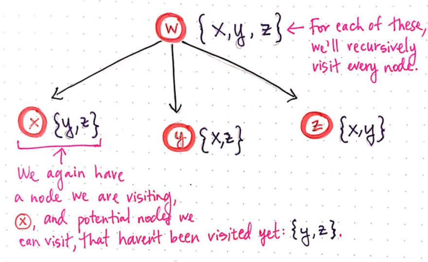
Notice that we’re starting to create a tree-like structure. For each of the potential nodes to visit from the starting node w, we now have three potential child “paths” that we could take. Again, for each of these three vertices, we’re keeping track of the node itself that we’re visiting as well as any potential nodes that we can visit next, which haven’t already been visited in that path.

Recursion is about repetition, so we’re going to do the same thing once again! The next step of recursion expands our tree once again.

Generating recursive calls for TSP, part 3.

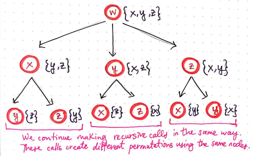
We’ll notice that, since each of the three nodes x, y, and z had two nodes that we could potentially visit next, each of them have spawned of two of their own recursive calls. We’ll continue to make recursive calls in the same way and, in the process, we’ll start to see that we’re creating different permutations using the same nodes.

We’ll notice that we’re now at the third level of recursive calls, and each node has only one possible place to visit next. We can probably guess what happens next – our tree is going to grow again, and each of the bottom-level nodes is going to spawn a single recursive call of its own, since each node has only one unvisited vertex that it can potentially check.

The image shown below illustrates the next two levels of recursive calls.

Generating recursive calls for TSP, part 4.

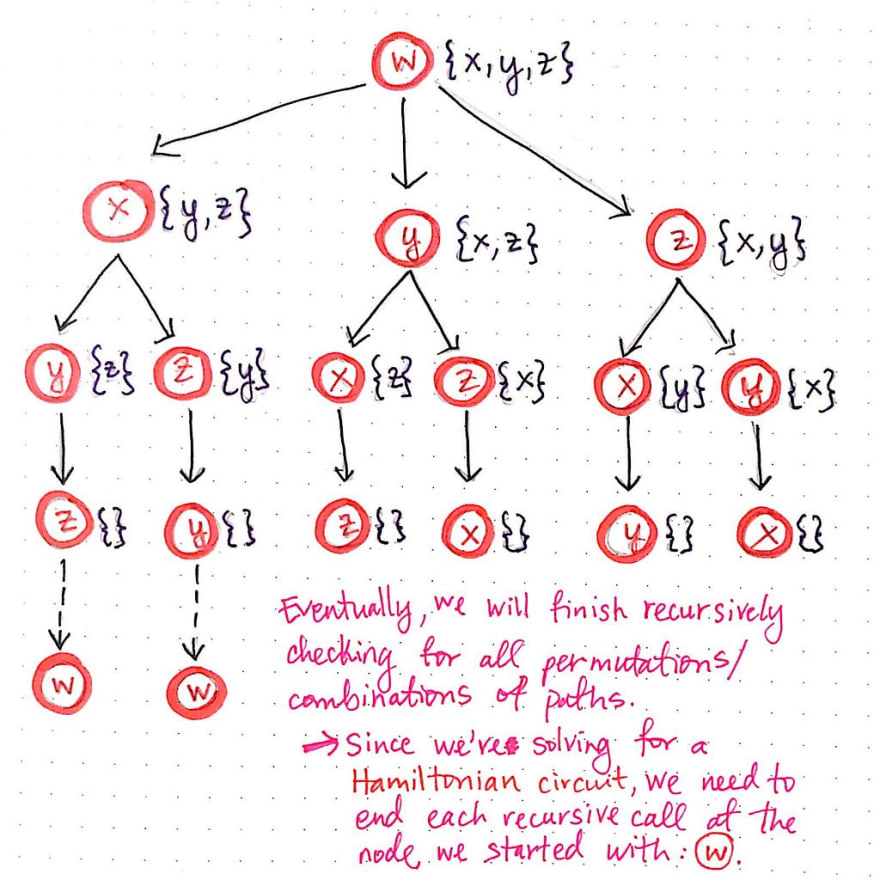
Notice that, when we get to the fourth level of child nodes, there is nowhere left to visit; every node has an empty list ({} ) of nodes that it can visit. This means that we’ve finished recursively checking for all permutations of paths.

However, since we’re solving for a Hamiltonian cycle, we aren’t exactly done with each of these paths just yet. We know we want to end back where we started at node w, so in reality, each of these last recurisvely-determined nodes needs to link back to vertex w.

Once we add node w to the end of each of the possible paths, we’re done expanding all of our permutations! Hooray! Remember how we determined earlier that every single of one of these potential routes is just a directed graph? All of those directed graphs have now revealed themselves. If we start from the root node, w, and work down each possible branch of this “tree”, we’ll see that there are six distinct paths, which are really just six directed graphs! Pretty cool, right?

So, what comes next? We’ve expanded all of these paths…but how do we know which one is the shorted one of them all?

We haven’t really been considering the cost or distance of this weighted graph so far, but that’s all about to change. Now that we’ve expanded this problem and found all of its possible permutations, we need to consider the total cost of each of these paths in order to find the shortest one. This is when an adjacency matrix representation of our original graph will come in handy. Recall that an adjacency matrix is a matrix representation of exactly which nodes in a graph contain edges between them. We can tweak our typical adjacency matrix so that, instead of just 1’s and 0’s, we can actually store the weight of each edge.

We can use an adjacency matrix to help us keep track of edge costs/distances.

Now that we have an adjacency matrix to help us, let’s use it to do some math – some recursive math, that is!

Mirror mirror on the wall, which is the shortest path of them all?

In order to determine which of these six possible paths is the shortest one – and thus the ideal choice for our salesman – we need to build up the cost of every single one of these paths.

Calculating recursive costs using recursion for TSP, part 1.

Since we’ve used recursion to expand these paths until we hit our base case of “no more nodes left to visit”, we can start to close up these recursive calls, and calculate the cost of each path along the way.

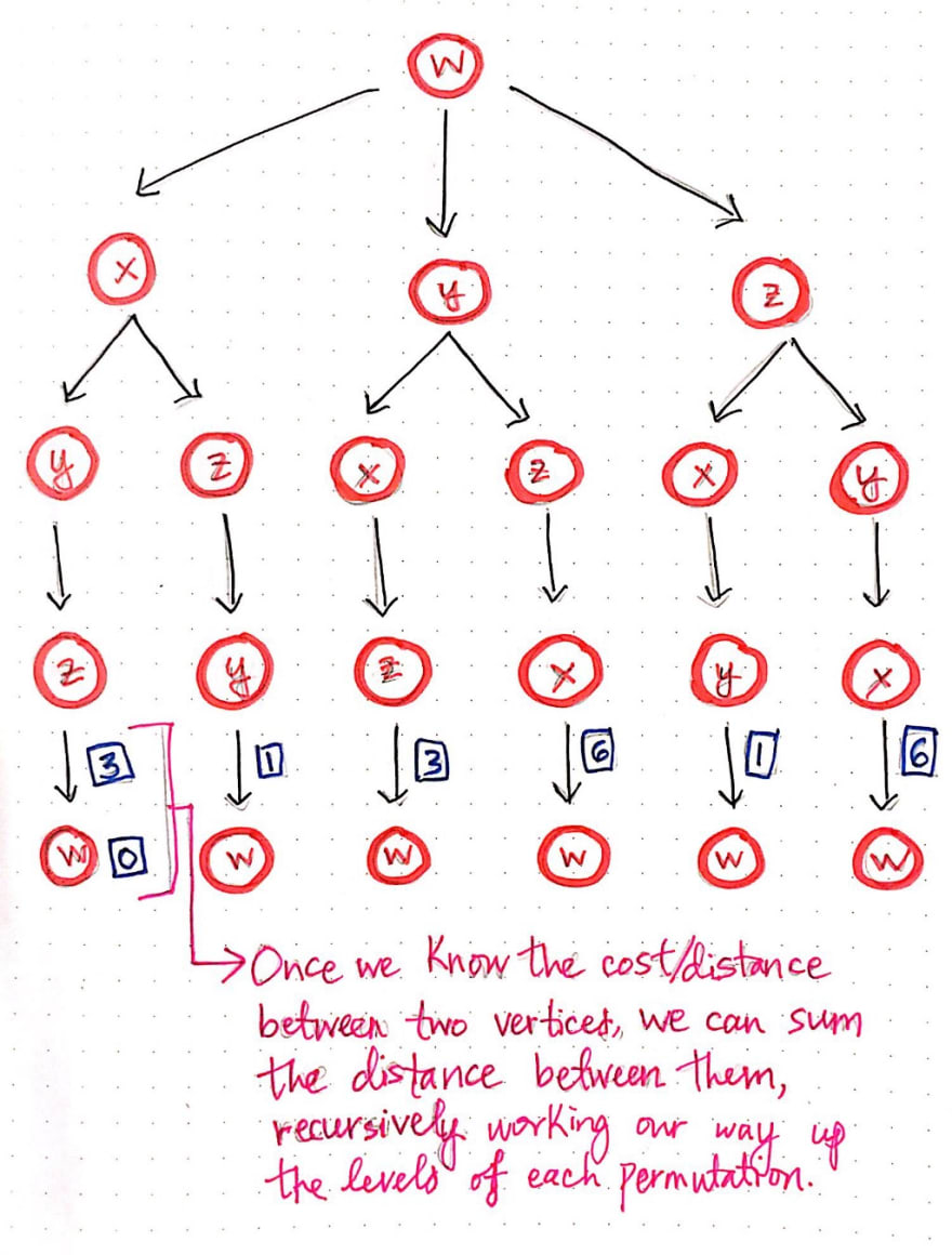
Once we know the cost between two vertices, we can sum the distance between them, and the remove the node from the tree. This will make more sense with an example, so let’s work our way from the lowest-level of this tree until we have found a solution for the shortest path.

We know that every single one of these branches – each of which represents a permutation of this particularly problem – ends with the node that we started on: node w. We’ll start with node w, and calculate the cost for our salesman to travel there.

Well, since our salesman starts at node w, the cost of traveling to node w is actually just 0. This makes sense if we think about it, because our salesman is already at that vertex, so it isn’t going to “cost” him anything to travel there! So, the math for the bottom level is pretty easy – the cost to get from w to w is 0. Next, we’ll apply the same technique again, but this time, we’ll move one level up.

Understanding the logic behind recursive addition for TSP.

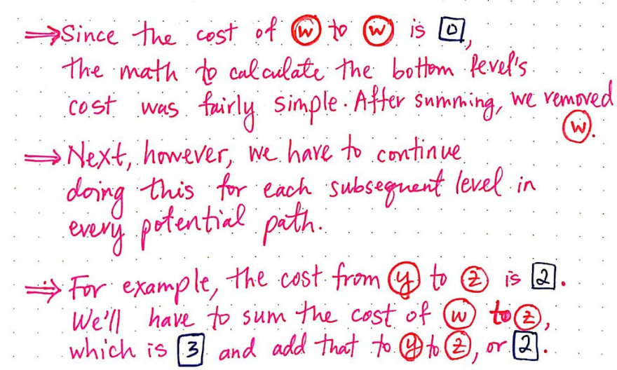
For example, if we refer to our adjacency matrix from the previous section, we’ll see that the cost of traveling from w to z is 3. Since we’re traveling from w –> w –> z, we can sum the distances between each of these vertices as we go. Traveling from w –> w is 0, and traveling from w –> z is 3, so we are essentially calculating 0 + 3. In a similar vein, the cost from z to y is 2. So, we will need to calculate w –> w –> z -> y, which is 0 + 3 + 2.

The drawing below illlustrates how this addition slowly works its way up the tree, condensing the recursive calls that built it up in the first place.

Calculating recursive costs using recursion for TSP, part 2.

Through this process, we’re effectively building up the cost or distance of each path, one level at a time, using our tree structure. Each time that we sum the distance between two nodes, we can remove the bottom node (the deeper of the two nodes being added together) from the tree, since we don’t need to use it anymore.

Calculating recursive costs using recursion for TSP, part 3.

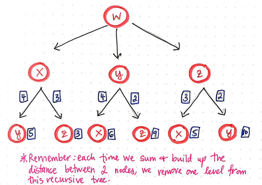
It is worth mentioning that we need to keep track of each of these paths , even after we finish doing the work of adding up their costs. For the sake of brevity, the paths themselves are not included in the illustrations shown here. However, it is crucial to keep track of which nodes were at the bottom of the tree – otherwise, we’d lose the entire path itself!

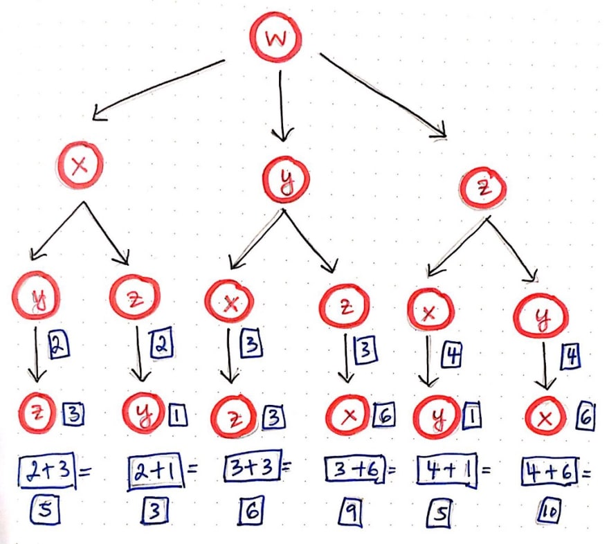
We will continue this process, but at some point, an odd thing is going to happen. In the next iteration of this recursive addition, we’ll notice that we come to an interesting fork in the road – literally! When we reach the third level and have condensed the bottom part of the tree, we have two possible options of how we can proceed with our additon.

Calculating recursive costs using recursion for TSP, part 4.

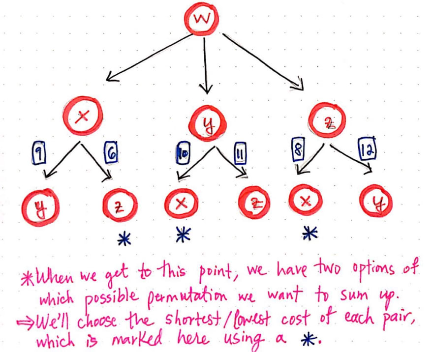
For example, looking at the child paths/branches from node x, we could either sum the distance from x to y, or we could sum the distance from x to z. So, how do we decide which one to choose?

Calculating recursive costs using recursion for TSP, part 5.

Our gut instinct would tell us that we’re looking for the shortest path, which probably means that we’ll want to choose the smaller of the two values. And that’s exactly what we’ll do! We’ll choose the path from z leading back to x, since the cost of that path is 6, which is definitely smaller than the path from y leading back to x, which is 9.

Once we’ve chosen the smallest of the two paths in our “fork in the road”, we are left with just three paths. All that’s left to do is to figure out the total cost of from x to w, y to w, and z to w. Referring to our adjacency matrix, we’ll see that these distances are 6, 1, and 3, respectively.

We can add these to the total costs of the paths that we’ve been recursively summing this whole time. In the illustration above, we’ll see that the three shortest paths that we’ve determined are actually noted down for convenience. As it turns out, there is one path that costs 12, and two paths that both cost 11. One of those travels from w to y, and takes the route of w -> y -> x -> z -> w, while the other travels from w to z, and takes the route of w -> z-> x -> u -> w.

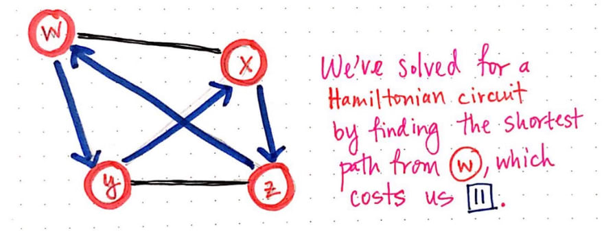
Since two of our three paths are equivalently small in size, it doesn’t really matter which one we choose; both of them are the “shortest path” in solving the traveling salesman problem.

And there we have it! We’ve solved for a Hamiltonian circuit by finding teh shortest path, with a distance/cost of 11, that starts and ends at node w.

We’ve solved for a Hamiltonian circuit!

Solving that was pretty awesome, right? It seemed super daunting at first, but as we worked through it, it got easier with each step. But here’s the thing: we had to take a lot of steps to do this. We knew from the beginning that we weren’t going to have the most elegant solution to this problem – we were just trying to get something working. But just how painful is the brute-force method, exactly?

Well, what if instead of a salesman who has to travel to four cities, we were trying to help out a salesman who had to travel to a whole lot more cities? What if the number of cities that they had to visit was n? How bad would our brute-force technique be?

Well, in our first example, n = 4. We’ll recall that, since we had already visited our first city (node w), we only had to make three recursive calls. In other words, we had to make 4 – 1, or n – 1 recursive calls.

Solving for n cities in the TSP.

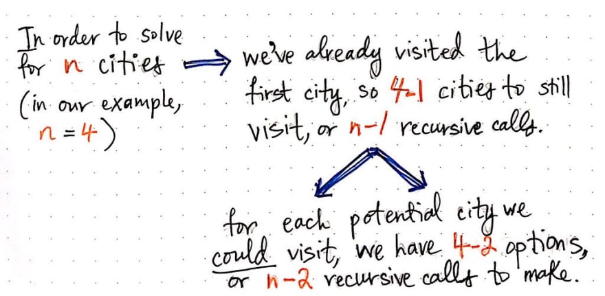
But, for each of those recursive calls, we had to spawn off two more recursive calls! That is to say, for each potential city that we could visit from the three nodes x, y, and z, we had 4 – 2 = 2 options of paths to take. In abstract terms, we’d effectively have n – 2 recursive calls at the next level of our tree.

Building up an unscalable “n factorial” problem.

If we continue figuring out this math, we’ll see that, at each level of the tree, we are basically on the path to finding a number that is going to be a factorial. To be more specific, we’re going to end up with n!, or n factorial.

Now, when we were dealing with a salesman who needed to visit just four cities, this really wasn’t too terrible of scenario to deal with. But, what happens when n is something much, much larger than 4? Most salesmen and women aren’t going to be traveling just to four cities; in almost every realistic case, n is going to be a much larger number!

The traveling salesman is not a fan of factorial algorithms!

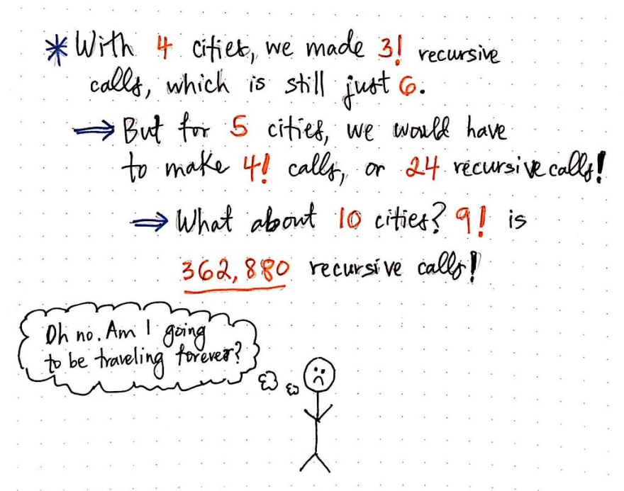
Well, to get a sense of how unscalable a factorial algorithm is, we needn’t increase the value of n by all that much. For example, when n = 4, we made 3! or 6 recursive calls. But if we had increased this only slightly so that n = 5, we would make 4! or 24 recursive calls, which would lead to a much, much larger tree. And what about when n = 10? That would result in 9! recursive calls, which is a really huge number: 362,880 to be exact. We probably can’t even imagine what would happen if our salesman had to travel to every city in the country, or even just 10 cities for that matter!

Surely, there must be a better way of helping our traveling salesman out so that he’s not traveling forever? Well, there certainly is. But more on that next week. In the meantime, someone should really tell this salesman about eBay – it would probably solve him a whole lot of heartache!

Resources

Unsurprisingly, there are many resources on the traveling salesman problem. However, not all of them are necessarily easy to understand! Some of them dive deep into the theory and mathematics of the problem, and it can be hard to find beginner-friendly content. Here are a few resources that are fairly easy to understand, and a good place to get started if you’re looking to learn more about TSP!

1. Travelling Salesman Problem, 0612 TV w/ NERDfirst
2. Coding Challenge #35.1: Traveling Salesperson, The Coding Train
3. History of TSP, University of Waterloo, Department of Mathematics
4. The Traveling Salesman problem, Professor Amanur Rahman Saiyed
5. A brief History of the Travelling Salesman Problem, Nigel Cummings
6. The Traveling Salesman Problem and Its Variation, Gregory Gutin and Abraham P. Punnen

---

Comments

[praveen075]

Are u yet to post the link for other programming approaches of TSP apart from Brute force method ? If present then will you please share the link below.

Good article.

Thanks.