If you spend enough time reading about programming or computer science, there’s a good chance that you’ll encounter the same ideas, terms, concepts, and names, time and again. Some of them start to become more familiar with time. Naturally, organically, and sometimes without too much effort on your part, you start to learn what all of these things mean. This happens because either you’ve slowly begun to grasp the concept, or you’ve read about a phrase enough times that you start to truly understand its meaning.
However, there are some ideas and definitions that are much harder to understand. These are the ones that you feel like you’re supposed to know, but you haven’t run across it enough to really comprehend it.
Topics that we feel like we’re meant to know – but never quite got around to learning – are the most intimidating ones of all. The barrier to entry is so high, and it can feel impossibly hard to understand something that you have little to no context for. For me, that intimidating topic is Dijkstra’s algorithm. I had always heard it mentioned in passing, but never came across it, so I never had the context or the tools to try to understand it.
Thankfully, in the course of writing this series, that has all changed. After years of fear and anxiety about Dijkstra’s algorithm, I’ve finally come to understand it. And hopefully, by the end of this post, you will too!
Graphs that weigh heavy on your mind
Before we can really get into Dijkstra’s super-famous algorithm, we need to pick up a few seeds of important information that we’ll need along the way, first.
Throughout this series, we’ve slowly built upon our knowledge base of different data structures. Not only have we learned about various graph traversal algorithms, but we’ve also taught ourselves the fundamentals of graph theory, as well as the practical aspects of representing graphs in our code. We already know that graphs can be directed, or undirected, and may even contain cycles. We’ve also learned how we can use breadth-first search and depth-first search to traverse through them, using two very different strategies.
In our journey to understand graphs and the different types of graph structures that exist, there is one type of graph that we’ve managed to skip over – until now, that is. It’s time for us to finally come face-to-face with the weighted graph!
A weighted graph is interesting because it has little to do with whether the graph is directed, undirected, or contains cycles. At its core, a weighted graph is a graph whose edges have some sort of value that is associated with them. The value that is attached to an edge is what gives the edge its “weight”.
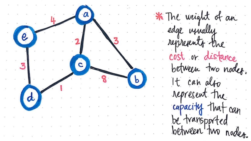
A common way to refer to the “weight” of a single edge is by thinking of it as the cost or distance between two nodes. In other words, to go from node a to node b has some sort of cost to it.
Or, if we think of the nodes like locations on a map, then the weight could instead be the distance between nodes a and b. Continuing with the map metaphor, the “weight” of an edge can also represent the capacity of what can be transported, or what can be moved between two nodes, a and b.
For example, in the example above, we could ascertain that the cost, distance, or capacity between the nodes c and b is weighted at 8.

The weighted-ness of the edges is the only thing that sets weighted graphs apart from the unweighted graphs that we’ve worked with so far in this series.
In fact, we probably already can imagine how we’d represent one of these weighted graphs! A weighted graph can be represented with an adjacency list, with one added property: a field to store the cost/weight/distance of every edge in the graph. Based on our previous research on graph representation, we’ll recall that the edges of a graph in an adjacency list live in the “list” portion.
For every single edge in our graph, we’ll tweak the definition of the linked list that holds the edges so that every element in the linked list can contain two values, rather than just one. These two values will be the opposite node’s index, which is how we know where this edge connects to, as well as the weight that is associated with the edge.
Here’s what that same example weighted graph would look like in adjacency list format.
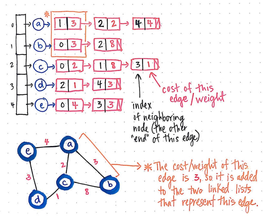
Right off the bat, we’ll notice two things about this graph representation: first, since it is an undirected graph, the edge between nodes a and b will appear twice – once in the edge list for node a and once in the edge list for node b. Second, in both instances that this edge is represented in either node’s respective edge list, there is a cost/weight that is stored in the linked list element that contains the reference to the neighboring node (in this case, either a or b).
Okay, so there’s nothing too wild that we need to wrap our heads around just yet, right?
Here’s where the weight of a graph starts to complicate things slightly:
finding the shortest path between two nodes becomes much trickier when we have to take into account the weights of the edges that we’re traversing through.
Let’s take a look at an example, and this will start to become more clear. In the simple directed, weighted graph below, we have a graph with three nodes (a, b, and c), with three directed, weighted edges.

Looking at this graph, we might be able to quickly determine – without much hesitation – the quickest way to get from node a to node b. There is an edge between a and b, so that must be the quickest way, right?
Well, not exactly. Taking the weights of these edges into account, let’s take a deeper, second look. If we take the route from node a to node b, it will “cost us” 5. However, if we take the route from node a to node c to node b, then it will cost us only 3.
But why 3? Well, even though it may intuitively seem like a longer path, if we sum up the edges of going from node a to c and then from node c to b, we’ll see that the total cost ends up as 2 + 1, which is 3. It might mean that we’re traveling through two edges, but a cost of 3 is certainly preferable to a cost of 5!
In our three-node example graph, we could fairly easily look at the two possible routes between our origin and destination nodes. However, what if our graph was much bigger – let’s say twenty nodes? It wouldn’t have been nearly as easy for us to find the shortest path, taking into account the weights of our weighted graph. And what if we were talking about an even bigger graph? In fact, most graphs that we deal with are far bigger than twenty nodes. How feasible and scalable and efficient would it be for us to use a brute-force approach to solving this problem?
The answer is that it’s not that feasible. Nor is it really any fun! And that’s where Dijkstra comes to the rescue.
Rules of Dijkstra’s game
Dijkstra’s algorithm is unique for many reasons, which we’ll soon see as we start to understand how it works. But the one that has always come as a slight surprise is the fact that this algorithm isn’t just used to find the shortest path between two specific nodes in a graph data structure. Dijkstra’s algorithm can be used to determine the shortest path from one node in a graph to every other node within the same graph data structure, provided that the nodes are reachable from the starting node.

This algorithm will continue to run until all of the reachable vertices in a graph have been visited, which means that we could run Dijkstra’s algorithm, find the shortest path between any two reachable nodes, and then save the results somewhere. Once we run Dijkstra’s algorithm just once, we can look up our results from our algorithm again and again – without having to actually run the algorithm itself! The only time we’d ever need to re-run Dijkstra’s algorithm is if something about our graph data structure changed, in which case we’d end up re-running the algorithm to ensure that we still have the most up-to-date shortest paths for our particular data structure.
So, how does Dijkstra’s algorithm actually work? It’s time to finally find out!
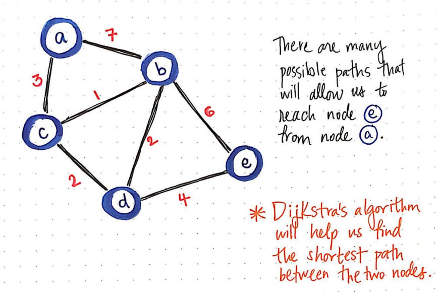
Consider the weighted, undirected graph above. Let’s say that we want to find the shortest path from node a to node e. We know that we’re going to start at node a, but we don’t know if there is a path to reach it, or if there are many paths to reach it! In any case, we don’t know which path will be the shortest one to get to node e, if such a path even exists.
Dijkstra’s algorithm does require a bit of initial setup. But, before we get to that, let’s take a quick look at the steps and rules for running Dijkstra’s algorithm. In our example graph, we will start with node a as our starting node. However, the rules for running Dijkstra can be abstracted out so that they can be applied to every single node that we’ll traverse through and visit in an effort to find the shortest path.
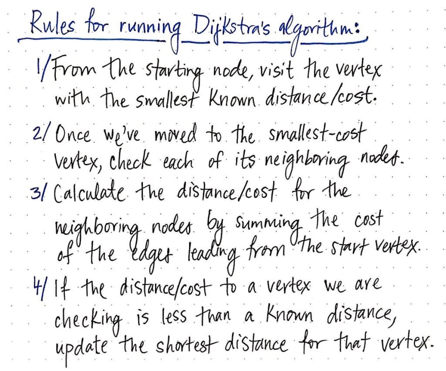
The abstracted rules are as follows:
- Every time that we set out to visit a new node, we will choose the node with the smallest known distance/cost to visit first.
- Once we’ve moved to the node we’re going to visit, we will check each of its neighboring nodes.
- For each neighboring node, we’ll calculate the distance/cost for the neighboring nodes by summing the cost of the edges that lead to the node we’re checking from the starting vertex.
- Finally, if the distance/cost to a node is less than a known distance, we’ll update the shortest distance that we have on file for that vertex.
These instructions are our golden rules that we will always follow, until our algorithm is done running. So, let’s get to it!
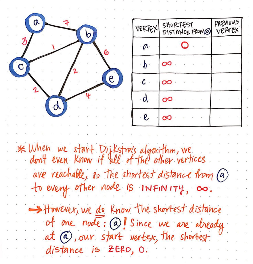
First things first: we need to initialize some things to keep track of some important information as this algorithm runs.
We’ll create a table to keep track of the shortest known distance to every vertex in our graph. We’ll also keep track of the previous vertex that we came from, before we “checked” the vertex that we’re looking at currently.
Once we have our table all set up, we’ll need to give it some values. When we start Dijkstra’s algorithm, we don’t know anything at all! We don’t even know if all of the other vertices that we’ve listed out (b, c, d, and e) are even reachable from our starting node a.
This means that, when we start out initially, the “shortest path from node a" is going to be infinity (∞). However, when we start out, we do know the shortest path for one node, and one node only: why, node a, our starting node, of course! Since we start at node a, we are already there to begin with. So, the shortest distance from node a to node a is actually just 0!
Now that we’ve initialized our table, we’ll need one other thing before we can run this algorithm: a way to keep track of which nodes we have or haven’t visited! We can do this pretty simply with two array structures: a visited array and an unvisited array.
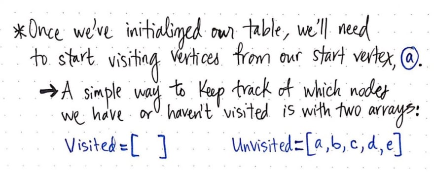
When we start out, we haven’t actually visited any nodes yet, so all of our nodes live inside of our unvisited array.
Okay, now we’re good shape! Let’s get started. Remember our four rules from earlier? We’re going to follow them, step-by-step, as we work through each vertex in this graph.
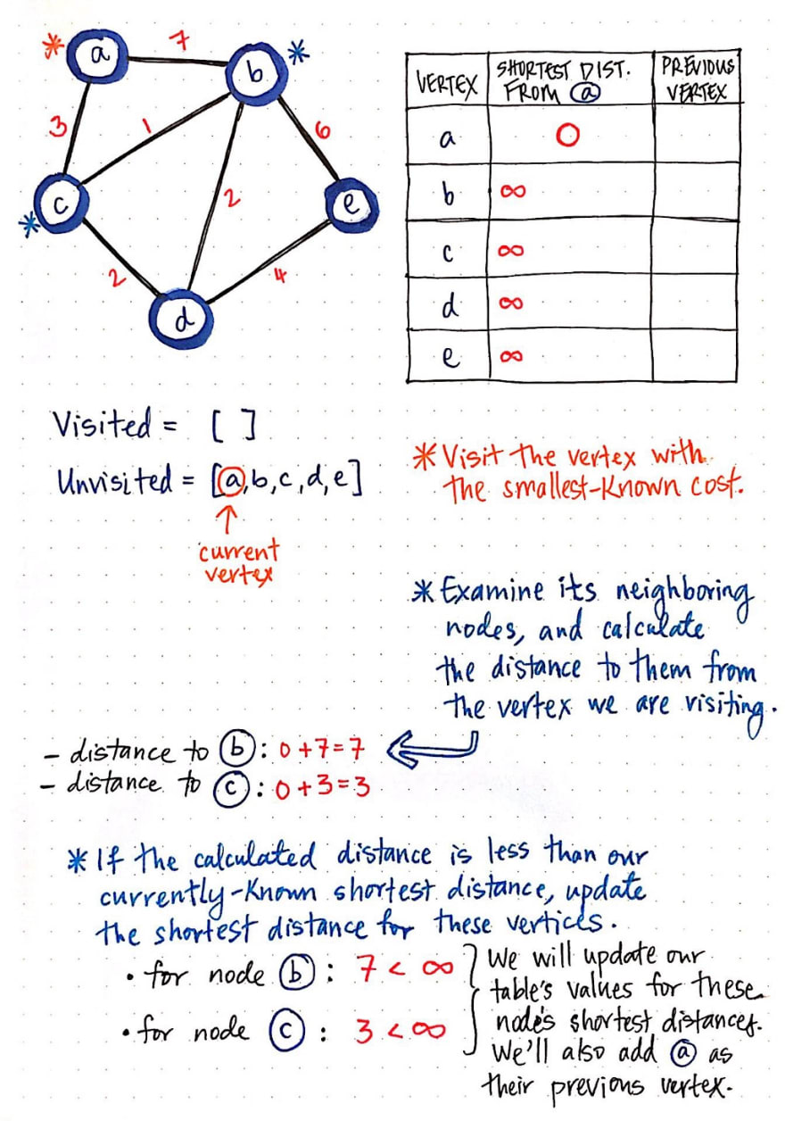
First, we’ll visit the vertex with the smallest-known cost/distance. We can look at the column that tells us the shortest distance from a. Right now, every vertex has a distance of infinity (∞), except for a itself! So, we’ll visit node a.
Next, we’ll examine it’s neighboring nodes, and calculate the distance to them from the vertex that we’re currently looking at (which is a). The distance to node b is the cost of a plus the cost to get to node b: in this case, 7. Similarly, the distance to node c is the cost of a plus the cost to get to node c: in this case, 3.
Finally, if the calculated distance is less than our currently-known shortest distance for these neighboring nodes, we’ll update our tables values with our new “shortest distance”. Well, currently, our table says that the shortest distance from a to b is ∞, and the same goes for the shortest distance from a to c. Since 7 is less than infinity, and 3 is less than infinity, we will update node b's shortest distance to 7, and node c's shortest distance to 3. We will also need to update the previous vertex of both b and c, since we need to keep a record of where we came from to get these paths! We’ll update the previous vertex of b and c to a, since that’s where we just came from.
Now, we’re done checking the neighbors of node a, which means we can mark it as visited! Onto the next node.
Again, we’ll look at the node with the smallest cost that hasn’t been visited yet. In this case, node c has a cost of 3, which is the smallest cost of all the unvisited nodes. So, node c becomes our current vertex.
We’ll repeat the same procedure as before: check the unvisited neighbors of node c, and calculate their shortest paths from our origin node, node a. The two neighbors of node c that haven’t been visited yet are node b and node d. The distance to node b is the cost of a plus the cost to get from node c to b: in this case, 4. The distance to node d is the cost of a plus the cost to get from node c to d: in this case, 5.
Now, let’s compare these two “shortest distances” to the values that we have in our table. Right now, the distance to d is infinity, so we’ve certainly found a shorter-cost path here, with a value of 5. But what about the distance to node b? Well, the distance to node b is currently marked as 7 in our table. But, we’ve found a shorter path to b, which goes through c, and has a cost of only 4. So, we’ll update our table with our shorter paths!
We’ll also need to add vertex c as the previous vertex of node d. Notice that node b already has a previous vertex, since we found a path before, which we now know isn’t actually the shortest. No worries – we’ll just cross out the previous vertex for node b, and replace it with the vertex which, as we now know, has the shorter path: node c.
Alright, so now we’ve visited both node a and c. So, which node do we visit next?
Again, we’ll visit the node that has the smallest cost; in this case, that looks to be node b, with a cost of 4.
We’ll check its unvisited neighbor (it only has one, node e), and calculate the distance to e, from the origin node, via our current vertex, b.
If we sum the cost of b, which is 4, with the cost that it takes to get from b to e, we’ll see that this costs us 6. Thus, we end up with a total cost of 10 as the shortest-known distance to e, from the starting vertex, via our current node.
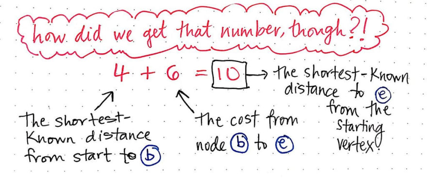
So, how did we get that number? It can seem confusing at first, but we can break it down into parts. Remember, no matter which vertex we’re looking at, we always want to sum the shortest-known distance from our start to our current vertex. In simpler terms, we’re going to look at the “shortest distance” value in our table, which will give us, in this example, the value 4. Then, we’ll look at the cost from our current vertex to the neighbor that we’re examining. In this case, the cost from b to e is 6, so we’ll add that to 4.
Thus, 6 + 4 = 10 is our shortest-known distance to node e from our starting vertex.
Behind the scenes of Dijkstra’s magic
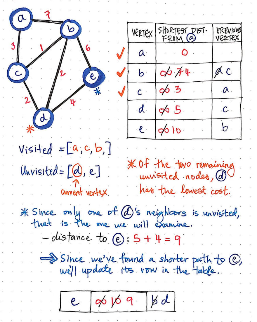
We’ll continue doing the same steps for each vertex that remains unvisited. The next node we’d check in this graph would be d, as it has the shortest distance of the unvisited nodes. Only one of node d's neighbors is unvisited, which is node e, so that’s the only one that we’ll need to examine.
When we sum the distance of node d and the cost to get from node d to e, we’ll see that we end up with a value of 9, which is less than 10, the current shortest path to node e. We’ll update our shortest path value and the previous vertex value for node e in our table.
Finally, we end up with just one node left to visit: node e.
However, it becomes pretty obvious that there’s nothing for us to really do here! None of node e's neighbors need to be examined, since every other vertex has already been visited.
All we need to do is mark node e as visited. Now, we’re actually completely done with running Dijkstra’s algorithm on this graph!
We’ve crossed out a lot of information along the way as we updated and changed the values in our table. Let’s take a look at a nicer, cleaner version of this table, with only the final results of this algorithm.

From looking at this table, it might not be completely obvious, but we’ve actually got every single shortest path that stems from our starting node a available here, right at our fingertips. We’ll remember that earlier, we learned that Dijkstra’s algorithm can run once, and we can reuse all the values again and again – provided our graph doesn’t change. This is exactly how that characteristic becomes very powerful. We set out wanting to find the shortest path from a to e. But, this table will allow us to look up all shortest paths!

The way to look up any shortest path in this table is by retracing our steps and following the “previous vertex” of any node, back up to the starting node.
For example, let’s say that we suddenly decide that we want to find the shortest path from a to d. No need to run Dijkstra’s algorithm again – we already have all the information we need, right here!
Using a stack data structure, we’ll start with node d, and push() it onto our stack. Then, we’ll look at node d's previous vertex, which happens to be node b. We’ll push() node b onto the stack. Similarly, we’ll look at node b' previous vertex (node c), and add that to our stack, and then look at node c's previous vertex, which is node a, our starting vertex!
Once we trace our steps all the way back up to our starting vertex, we can pop() each vertex off of the stack, which results in this order: a – c – b – d. As it turns out, this is the exact path that will gives us the lowest cost/distance from node a to node d! Pretty rad, right?

In many ways, Dijkstra’s algorithm is a sophisticated take on the typical form of breadth-first graph traversal that we’re already familiar with. The major differences are the fact that it is a bit smarter, and can handle weighted graphs very well. But, if we look at Dijkstra’s algorithm visualized, like the animation shown here, we’ll see that it basically functions like a BFS search, spreading out wide rather than pursuing one specific path deeply.
The most common example of Dijkstra’s algorithm in the wild is in path-finding problems, like determining directions or finding a route on GoogleMaps.

However, to find a path through GoogleMaps, an implementation of Dijkstra’s algorithm needs to be even more intelligent than the one that we created today. The version of Dijkstra’s algorithm that we implemented here is still not as intelligent as most forms that are used on a practical level. Imagine not just a weighted graph, but also having to calculate things like traffic, road conditions, road closures, and construction.
If this all feels like a lot to take in, don’t worry – it’s complicated stuff! In fact, it’s a hard problem that even Dijkstra struggled to exemplify well. As it turns out, when Edsger W. Dijkstra was first thinking about the problem of finding the shortest path back in 1956, he had a difficult time trying to find a problem (and its solution) that would be easy to understand for people who did not come from the computing world! He eventually did come up with a good example problem to showcase the importance of being able to find a shortest path. He chose – you guessed it! – a map as an example. In fact, when he designed his algorithm originally, he implemented it for a computer called the ARMAC. He used the example of a transportation map, which contained cities from across the Netherlands, in order to showcase how his algorithm worked.
Towards the end of his life, Dijkstra sat down for an interview and revealed the full backstory how he came up with his now-famous algorithm:
What is the shortest way to travel from Rotterdam to Groningen? It is the algorithm for the shortest path which I designed in about 20 minutes. One morning I was shopping with my young fiancée, and tired, we sat down on the café terrace to drink a cup of coffee and I was just thinking about whether I could do this, and I then designed the algorithm for the shortest path.
So what’s the moral of the story? I’m pretty sure it’s as simple as this: there is no problem that can’t be solved with a nice cup of coffee.
Resources
For better or for worse, Dijkstra’s algorithm is one of the most well-known methods of graph traversal in the world of computer science. The bad news is that sometimes it can feel intimidating to try to understand how it works, since there are so many references to it. The good news is that there are plenty of resources out there – you just need to know which ones to start with! Here are some of my favorites.
- Graph Data Structure – Dijkstra’s Shortest Path Algorithm, Kevin Drumm
- Dijkstra’s Algorithm, Computerphile
- Dijkstra’s Shortest Paths Algorithm for Graphs, Sesh Venugopal
- A Single-Source Shortest Path algorithm for computing shortest path, Professor Ileana Streinu
- A Note on Two Problems in Connexion with Graphs, E.W. Dijkstra






Top comments (4)
Hi!
Great article, but you accidentally changed the previous vertex of node d when you were visiting node e, resulting in a not quite correct shortest path from a to d later on.
Thanks for your work, your posts are really good!
I created this challenge in Go, to find a shortest path for word ladder. Here is an implementation - github.com/plutov/practice-go/tree...
This is such an awesome, well thought out and detailed article. Thank you very much for it and the work you put into it!