Introduction to Music Information Retrieval Pt. 1

I love music. I listen to it all day at work, I can play it, and (sometimes) I can make it. I also love analyzing stuff like congressional elections or exploring age of first birth. So, why not try and combine those two things and analyze some of the music in my iTunes library?

Motivation

Spotify knows my music tastes better than I do, and 9 times out of 10, their curated playlists made for me are absolutely spot on. I though that I'd like to try and replicate some of what they have done from a first principles perspective.

I began by looking in to the Spotify API and trying to figure out how to replicate their results in their audio analysis GET route. I was then lead to this reddit discussion where a search keyword given was Subject Audio Classification. My Google Fu then led me to this god send of a site https://musicinformationretrieval.com/. This site has tons of great resources, and also links to the International Society of Music Information Retrieval that has loads of great research papers. A lot of the following examples are based off of the lessons there.

My main objective is to help other people clarify what it is they should be looking for when analyzing music, as well as some tools to help get them started.

What you'll need

I work on macOSX with High Sierra installed. I run an anaconda distribution with python 2.7.13.
For this notebook, all that you'll need are numpy librosa matplotlib and Ipython. If you try to load a song with librosa and it does not work, you may need to install ffmpeg using homebrew.

Getting Started: Initial Challenges and Solutions

Embarking on this project was extremely frustrating for a long time. I did not know what keywords I should google (feature extraction on audio data?) and there were only 1 or 2 tutorials that specifically dealt with voice classification or ambient sound. Furthermore, within the tutiorials, there was no interpretation or explanation of any of the features that were being extracted, and they were very technical terms. Another huge challenge in this space is copyright laws for songs. There aren't huge repositories of pop song mp3s lying around nor are music file formats standardized in any way.

So how did I get around these challenges?

• For tools: First thing I found was in the way of Python was Librosa. I immediately started trying to read .m4a files from my iTunes library, but my computer threw a fit. Install ffmpeg using homebrew. Now I could actually read files on my computer.
• For songs, I used what I have on my own computer. There are other sources that you can find with raw audio data, although many others leave out the raw files for reasons above.
• As far as interpreting features goes, I had to go back to the basics! That's what I'd like to start with :)

Basic Terms and Concepts of Signal Processing

There were a lot of terms that I came across that I was pretty familiar with, but definitely needed some refreshing.

Cycle: Also known as a period. How many radians it takes for a to repeat itself. For sine, this is 2$\pi$ radians. More practically, if a heart beats once every 30 seconds, we say that it's period is 30 seconds

Hertz: (Not the car rental company). 1 hertz = 1 cycle per a second. 440 Hz means 440 cyles/second.

Frequency: How many cycles per a unit of time a signal repeats itself. It is the inverse of cycle. If my heart beats once every half second (cycle), then my frequency is 120 beats per a minute.

Signal: The actual timeseries of frequencies at a point in time from a file. We use librosa.load('filename.mp3', sr=our_sampling_rate) to load a file in to a audio timeseries.

Sampling Rate: The rate at which a sample is taken from an audio file. Defaults to 22050. If you multiply it by some a unit of time, you get the number of samples taken in that time.

Energy: Formally, the area under the squared magnitude of the signal. Roughly corresponds to how load the signal is.

Fourier Transform: This is a hugely important operation in signal processing. While the math of it is pretty dense, what it does is fairly intuitive. It breaks down a signal in to its constituent frequencies that make it up. In other words, it takes something that exists in a time domain (signal) and maps it in to the frequency domain, where the y-axis is magnitude. It's very similar to how a musical chord can be broken down in to the separate notes that make it up, i.e. a C triad chord is composed of the notes C, E, and G.

Now that we have some basic terminology down, let's go through some simple examples that use these terms.

from __future__ import division
import numpy as np
import seaborn as sns
%matplotlib inline
import matplotlib.pyplot as plt
plt.rcParams['figure.figsize'] = (12,8)

import librosa.display
import IPython.display as ipd

Lets create a simple audio wave that is 440 HZ (A note above middle C, specifically A4) that lasts for 3 seconds. This will be a pure tone. We'll use numpy.sin to construct the sine wave. Recall from high school physics/trig that the formula for a sin wave is $A* sin(2*{\pi}*R)$ where R is radians and A is amplitude. We can get the number of radians by multiplying a frequency (radians/time) by the time variable.

sr = 22050 # sample rate
T = 3.0    # seconds
t = np.linspace(0, T, int(T*sr), endpoint=False) # time variable, evenly split by number of samples within timeframe
freq = 440 #hz A4
amplitude = 0.5

# synthesize tone
signal = amplitude * np.sin(2 * np.pi * freq * t) # from our formula above
print "there are " + str(signal.shape[0]/T) + " \
samples of audio per second, if T was 2 seconds, the shape would be " + str(signal.shape[0]*2)

there are 22050.0 samples of audio per second, if T was 2 seconds, the shape would be 132300

Let's play the tone!

ipd.Audio(signal, rate=sr) #

If we plot the entire time series, then it just looks like 1 solid mass because of the high frequency. Instead, let's plot a small sample of the tone so that we can see only two periods.

# sr / freq = # of frames in one period,
two_periods = int(2 * (sr / freq))

librosa.display.waveplot(signal[:two_periods + 1], sr=sr);

Lets make a tone with a much lower frequency

sr = 22050 # sample rate
T = 2.0    # seconds
t = np.linspace(0, T, int(T*sr), endpoint=False) # time variable, 
freq = 110 #hz 
amplitude = 1

# synthesize tone
low_signal = amplitude*np.sin(2*np.pi*freq*t)

You might not be able to play this tone through your computer speakers, try headphones if nothing plays.

ipd.Audio(low_signal, rate=sr) # BASS

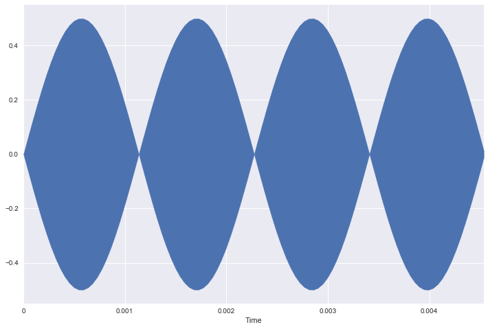
Since there are 22050 samples in this signal with a frequency of 110 hz, that means if we divide the number of samples by the frequency, we should be able to see how many frames are in one period of the signal and plot the single period.

# 22050 / 110 = 200.45 => round up to 201
plt.plot(t[:201], low_signal[:201])
plt.show()

To help our own intuition, lets look at how the two signals are related to each other. Since 110 hz is about a quarter the frequency of 440 hz, then 4 periods of higher frequency signal should fit in 1 period of the lower frequency. Green is the higher frequency.

librosa.display.waveplot(low_signal[:4*two_periods], sr=sr);
librosa.display.waveplot(signal[:4*two_periods], sr=sr);

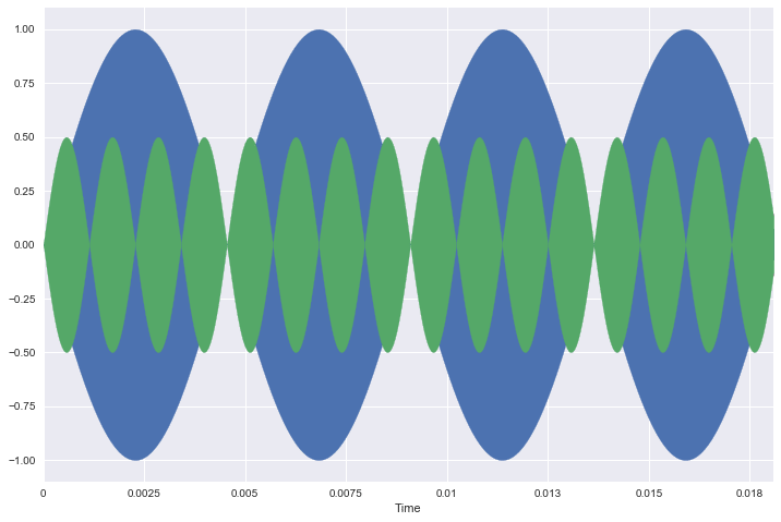
Alright awesome! We've been able to construct our own sound waves and get an idea of the how frequency affects the tone.

Load your own music!

Instead of synthesizing our own tones, lets load a small sample of a song from your music library and take a look at it!

# read 4 seconds of this song, starting at 6 seconds
music_dir = '/Users/benjamindykstra/Music/iTunes/Led Zeppelin/Led Zeppelin IV/02 Rock & Roll.m4a'
data, sr = librosa.load(music_dir, offset=6.0, duration=4.0)

ipd.Audio(data, rate=sr)

librosa.display.waveplot(data, sr=sr); # it just looks loud!

Fourier Transform

Lets see what happens if we take the fast fourier transform of our original signal (440 hz). I expect that there will be a single line at 440 hz mark on the x-axis. After we do our simple case, we can also break down our small song clip.

import scipy

X = scipy.fft(signal)
X_mag = np.absolute(X)
f = np.linspace(0, sr, len(X_mag)) # frequency variable

plt.plot(f[1000:2000], X_mag[1000:2000]); # magnitude spectrum
plt.xlabel('Frequency (Hz)');

Look at that! a single spike right at 440 Hz. Warms me heart :)

Now we can take a quick look at Rock & Roll.

rr_fft = scipy.fft(data)
rr_mag = np.absolute(rr_fft)
f = np.linspace(0, sr, len(rr_mag)) # frequency variable
plt.plot(f, rr_mag) # magnitude spectrum
plt.xlabel('Frequency (Hz)')
plt.title('Rock and Roll Babay');

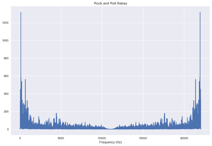
The reason that the Fourier transform is so important to us, is that it allows us to analyze the occurrence and power of each frequency through a whole song. If we break up a song in to parts, we can start to look at how the distribution changes over the course of the song. We can also use it to separate harmonic and percussive components of a signal. It is a fundamental building block of any algorithms or features that utilize frequency analysis.

Thanks for following along! In my next post we'll get in to the weeds with segmentation and feature extraction with lots of explanations.