

Introduction
It's always vital to know what to do while cleaning data so that you can get correct insights from it. Data that isn't accurately cleansed for analysis can produce false results, as well as prevent your model from generalizing properly when tested with new data.
In this article, we'll go through the four things you should do every time you clean data so it's ready for analysis and predictions.
Let's get this party started.
Prerequisite
- Make sure you have your environment set up (i.e. you must have a jupyter notebook)
Have pandas library installed on your notebook.
Have Seaborn library installed on your notebook.
Have Numpy library installed on your notebook.
What is Data Cleansing?
The process of finding and fixing inaccurate data from a dataset or data source is known as data cleaning. In simple terms, it refers to the process of preparing your data for exploratory data analysis (EDA).
Now that we've understood what data cleaning entails, we can begin working on the four items necessary to prepare the data for EDA.
So, due to proprietary issues, I won't be able to disclose the datasets that we'll be utilizing in this article, but I'll provide screenshots so we can see what's going on.
These are the four things to do when you want to clean your data for analysis and predictions.
Note: make sure you have imported these two libraries into your environment.
import pandas as pd
import seaborn as sns
import numpy as np
1. Dealing with missing values
The first thing as a data scientist/analyst is to always check the info of your data for missing values. To do this type the following code
df = pd.read_csv(file_path) #Input the filepath

df.info()
In the case of my file, this is my screenshot.
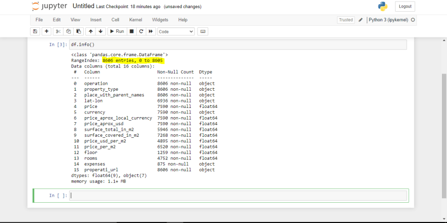
We can see from the above image (the annotation part) that we have 8606 entries. Now looking at the columns/features in the dataframe we can see obviously that we have missing values. The next thing for us is to deal with those missing values.
Now this is where the question comes
How can we deal with missing values?
When it comes to data that isn't Time-Series (I will talk about that in another article). There are two ways to go about it.
Dropping the values.
Imputation.
Dropping values
The only time you should drop values in a dataframe is if more than 60% of the observations are missing. So, if you review the dataframe and discover that 60% of the data is missing, it may be wise to drop the column with that missing value if you think it is unnecessary. If you want to drop those observations you can type
Another thing to consider is if you're building a model to predict something and you discover that the target column (i.e. this is the column you want to forecast) has missing values. You must remove all missing values from the target column, which will have an impact on other columns as well.
So in our case now our target column("price_usd_per_m2") has missing values so we have to drop those values. To do that we have to type:
df.dropna(subset = ["price_usd_per_m2"], inplace=True)
Now let's check the info of our data frame.
df.info()

We can now observe that our dataframe has shrunk from 8606 to 4895 entries. However, as you can see, there are still some missing values. Now let's have a look at the two criteria for dealing with missing data. We can see that the first criteria, Dropping values, applies to some of our columns which are floor and expenses the best thing to do is to drop those columns away(though it is not advisable to drop the floor column, bit for the case article we'll have to drop it).
df.drop(columns = ["floor", "expenses"], inplace=True)

We can see that we still have some missing values, but they are not up to 60% so we move to the other types of dealing with missing values.
Imputation
When it comes to the imputation of missing data, the most common method is to use the mean value of all the total values in the column. However, there are several guidelines for when you should not use mean which I will outline below. They are as follows:
-If your column contains values with different variances, such as positive and negative numbers, you should not utilize mean.
-If your column contains just binary values of 1s and 0s, you should avoid using the mean approach.
If your columns as the following features it is advisable to drop those observations.
Note don't confuse observation with a column. Observation means row so if you want to drop rows you make use of the following code
df.dropna(subset=[""], inplace=True)
As previously stated, this approach does not work with time-series data. It has a different approach to dealing with missing values, which I'll cover in a later article.
Also note it is always advisable to fill a column that has numeric missing values such as float and integer.
Now back to our dataset since our dataset does not have the above criteria I'm going to use the mean approach and I have only 1 numeric column(which is room) that has missing values. So I'm going to fill it with the mean value of the total values. To do that type the below code.
df.fillna(np.mean(df["rooms"], inplace=True)

Now that we don't have numerical columns that have missing values we are good to go.
2. Checking for Multicollinearity
Multicollinearity is a statistical concept in which independent variables in a feature matrix (which includes all variables in the dataframe except the target variable) are correlated. Now that we've understood what multicollinearity is. Let's check it out
Back to our dataframe since price_aprox_usd is our target value we are going to copy drop it (what this means is I'm going to pass in the drop attribute without using inplace parameter) so it will return a copy of it. So to see the multicollinearity type this:
df.drop(columns = "price_aprox_usd").corr()
Notice that I didn't pass in inplace so it returns a copy of the data frame without price_usd_per_m2 and also notice the
.corr()attribute it is used to find the correlation.
After you run the above you should have something like this.

Now that we've seen the correlation numerically it will be nice to visualize so we can know what's going on. So we will be using seaborn. Just save the above code into a variable vis_corr. Check below to see what I mean.
vis_corr = df.drop(columns = "price_aprox_usd").corr()
Now to visualize it we will use seaborn just type the following code to see the visualization.
sns.heatmap(vis_corr);
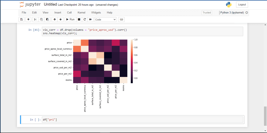
So let's unpack what's going on here. The diagram above shows the level of correlation among different features in the dataframe. However, if we have features in which their correlation value is greater than 0.5 it means those features are highly correlated with one another.
Now that we've understood that we can see that price, price_aprox_local_currency are correlated with one another. Also surface_total_in_m2 and surface_covered_in_m2 are also very correlated. So we have to drop one of those features.
The issue now is "how do we know which feature to drop now that we've noticed the concerns with multicollinearity in our dataframe?"
To figure out which feature to eliminate, we'll need to look at the association between each of these features and our target variable. After we've done that then the feature with the highest correlation value will be the one to be dropped. Please see the code below to understand what I'm saying, and I'll also include the correlation value for each variable as a comment.
df["price"].corr(df["price_aprox_usd"]) #corr_value = 0.68

df["price_aprox_local_currency"].corr(df["price_aprox_usd"]) #corr_value = 1.0

df["surface_covered_in_m2"].corr(df["price_aprox_usd"]) #corr_value = 0.13

df["surface_total_in_m2"].corr(df["price_aprox_usd"]) #corr_value=0.21
Okay now that we've seen the correlation values of all the features so the features that have to be dropped are price_aprox_local_currency and surface_covered_in_m2.
I will be dropping surface_covered_in_m2 rather than surface_total_in_m2. I feel like the adjective "total" makes it have more information well.
So to speak there might be sometimes in which you have to go for the one which has the lowest value. But based on my preference I choose to drop surface_covered_in_m2
So to do that we have to type
df.drop(columns = ["price_aprox_local_currency", "surface_covered_in_m2"], inplace=True)
Okay so having done that we are good to go. Let us look at another core thing we need to look at.
3. Dealing with leaky features
To understand what leaky features are. Consider the following scenario: you were scheduled to take an exam for which you had not prepared, but you were fortunate enough to see the answers to the exam questions before entering the room. How will you perform as opposed to you didn't see the answers at all? You will pass all the exams right!. That is what leaky features are also. They're features that fool the model into thinking it's some kind of geek who can predict anything unusual, while, when it comes to predicting data that hasn't been seen before, the model will completely fail.
So back to our dataframe let's check maybe we have any leaky features in our data frame.
df.info()

So in our dataframe we can see that we have leaky features in it. Our leaky features are the price, price_usd_per_m2, price_per_m2. We can see that these features are cheats to our dataframe considering that we want to build a model that can predict house prices. It will be very stupid to have prices columns again in our dataframe. These columns are cheats to our target variable which is price_aprox_usd. We have to drop them from our dataframe.
df.drop(columns = "price_usd_per_m2", "price_per_m2", inplace=True)
Now that we are done we are good to go. So let's look at the last core thing we need to focus on when building a predictive model.
4. Dropping high and low cardinality categorical variables.
A cardinality categorical variable (e,g places, names, emails, etc.) is said to be low or high when it has few or many unique numbers of value.
So for us to be able to check the cardinality of our categorical variable which are most types of object datatype. We will use the following code.
df.select_dtypes("O").nunique()
After running the code we can see that we have 1 low and high cardinality variable which are operation and properati_url. So we have to drop them. The essence of dropping the cardinality variable is that it will cause insanity in our model which we don't want.
df.drop(columns = ["operation", "properati_url"], inplace=True)

Conclusion
So we have gotten to the end of our journey, there are still other core things to look at when cleaning the data like dealing with outliers and other kinds of stuff. Thank you for reading. I'm open to suggestions, feedback, and where I need to improve on the article. You can follow me for more articles.Thanks

Oldest comments (0)