We’ll be analyzing stock data with Python 3, pandas and Matplotlib. To fully benefit from this article, you should be familiar with the basics of pandas as well as the plotting library called Matplotlib.
Time series data
Time series data is a sequence of data points in chronological order that is used by businesses to analyze past data and make future predictions. These data points are a set of observations at specified times and equal intervals, typically with a datetime index and corresponding value. Common examples of time series data in our day-to-day lives include:
- Measuring weather temperatures
- Measuring the number of taxi rides per month
- Predicting a company’s stock prices for the next day
Variations of time series data
- Trend Variation: moves up or down in a reasonably predictable pattern over a long period of time.
- Seasonality Variation: regular and periodic; repeats itself over a specific period, such as a day, week, month, season, etc.
- Cyclical Variation: corresponds with business or economic ‘boom-bust’ cycles, or is cyclical in some other form
- Random Variation: erratic or residual; doesn’t fall under any of the above three classifications.
Here are the four variations of time series data visualized:

Importing stock data and necessary Python libraries
To demonstrate the use of pandas for stock analysis, we will be using Amazon stock prices from 2013 to 2018. We’re pulling the data from Quandl, a company offering a Python API for sourcing a la carte market data. A CSV file of the data in this article can be downloaded from the article’s repository.
Fire up the editor of your choice and type in the following code to import the libraries and data that correspond to this article.
Example code for this article may be found at the Kite Blog repository on Github.
# Importing required modules
import pandas as pd
import numpy as np
import matplotlib.pyplot as plt

# Settings for pretty nice plots
plt.style.use('fivethirtyeight')
plt.show()

# Reading in the data
data = pd.read_csv('amazon_stock.csv')
A first look at Amazon’s stock Prices
Let’s look at the first few columns of the dataset:
# Inspecting the data
data.head()
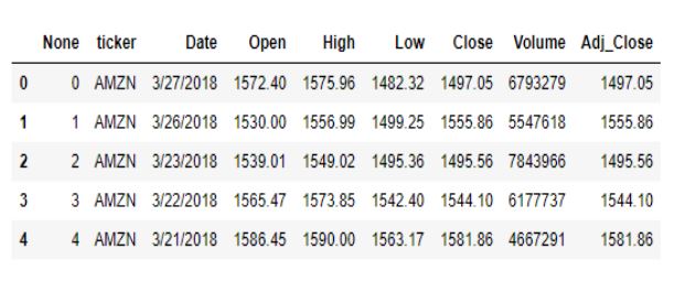
Let’s get rid of the first two columns as they don’t add any value to the dataset.
data.drop(columns=['None', 'ticker'], inplace=True)
data.head()

Let us now look at the datatypes of the various components.
data.info()
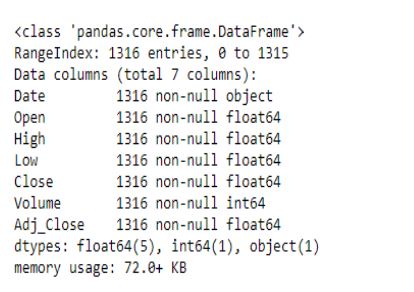
It appears that the Date column is being treated as a string rather than as dates. To fix this, we’ll use the pandas to_datetime() feature which converts the arguments to dates.
# Convert string to datetime64
data['Date'] = data['Date'].apply(pd.to_datetime)
data.info()
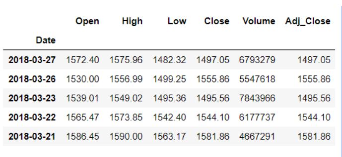
Lastly, we want to make sure that the Date column is the index column.
data.set_index('Date', inplace=True)
data.head()
Now that our data has been converted into the desired format, let’s take a look at its columns for further analysis.
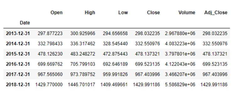
- The Open and Close columns indicate the opening and closing price of the stocks on a particular day.
- The High and Low columns provide the highest and the lowest price for the stock on a particular day, respectively.
- The Volume column tells us the total volume of stocks traded on a particular day.
The Adj_Close column represents the adjusted closing price, or the stock’s closing price on any given day of trading, amended to include any distributions and/or corporate actions occurring any time before the next day’s open. The adjusted closing price is often used when examining or performing a detailed analysis of historical returns.
data['Adj_Close'].plot(figsize=(16,8),title='Adjusted Closing Price')
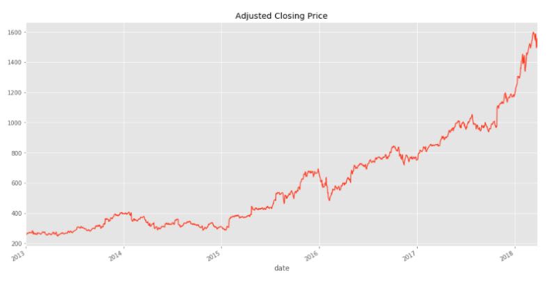
Interestingly, it appears that Amazon had a more or less steady increase in its stock price over the 2013-2018 window. We’ll now use pandas to analyze and manipulate this data to gain insights.
Pandas for time series analysis
As pandas was developed in the context of financial modeling, it contains a comprehensive set of tools for working with dates, times, and time-indexed data. Let’s look at the main pandas data structures for working with time series data.
Manipulating datetime
Python’s basic tools for working with dates and times reside in the built-in datetime module. In pandas, a single point in time is represented as a pandas.Timestamp and we can use the datetime()function to create datetime objects from strings in a wide variety of date/time formats. datetimes are interchangeable with pandas.Timestamp.
from datetime import datetime
my_year = 2019
my_month = 4
my_day = 21
my_hour = 10
my_minute = 5
my_second = 30
We can now create a datetime object, and use it freely with pandas given the above attributes.
test_date = datetime(my_year, my_month, my_day)
test_date


# datetime.datetime(2019, 4, 21, 0, 0)
For the purposes of analyzing our particular data, we have selected only the day, month and year, but we could also include more details like hour, minute and second if necessary.
test_date = datetime(my_year, my_month, my_day, my_hour, my_minute, my_second)
print('The day is : ', test_date.day)
print('The hour is : ', test_date.hour)
print('The month is : ', test_date.month)

# Output

The day is :  21
The hour is :  10
The month is :  4
For our stock price dataset, the type of the index column is DatetimeIndex. We can use pandas to obtain the minimum and maximum dates in the data.
print(data.index.max())
print(data.index.min())

# Output

2018-03-27 00:00:00
2013-01-02 00:00:00
We can also calculate the latest date location and the earliest date index location as follows:
# Earliest date index location
data.index.argmin()
#Output
1315
# Latest date location
data.index.argmax()
#Output
0
Time resampling
Examining stock price data for every single day isn’t of much use to financial institutions, who are more interested in spotting market trends. To make it easier, we use a process called time resampling to aggregate data into a defined time period, such as by month or by quarter. Institutions can then see an overview of stock prices and make decisions according to these trends.
The pandas library has a resample() function which resamples such time series data. The resample method in pandas is similar to its groupby method as it is essentially grouping according to a certain time span. The resample() function looks like this:
data.resample(rule = 'A').mean()
To summarize:
-
data.resample()is used to resample the stock data. - The ‘A’ stands for year-end frequency, and denotes the offset values by which we want to resample the data.
-
mean()indicates that we want the average stock price during this period.
The output looks like this, with average stock data displayed for December 31st of each year
Below is a complete list of the offset values. The list can also be found in the pandas documentation.
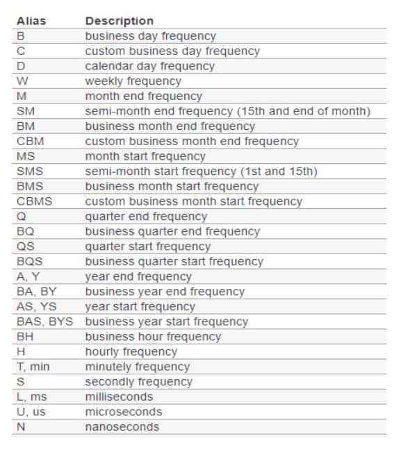
Offset aliases for time resampling
We can also use time sampling to plot charts for specific columns.
data['Adj_Close'].resample('A').mean().plot(kind='bar',figsize = (10,4))
plt.title('Yearly Mean Adj Close Price for Amazon')
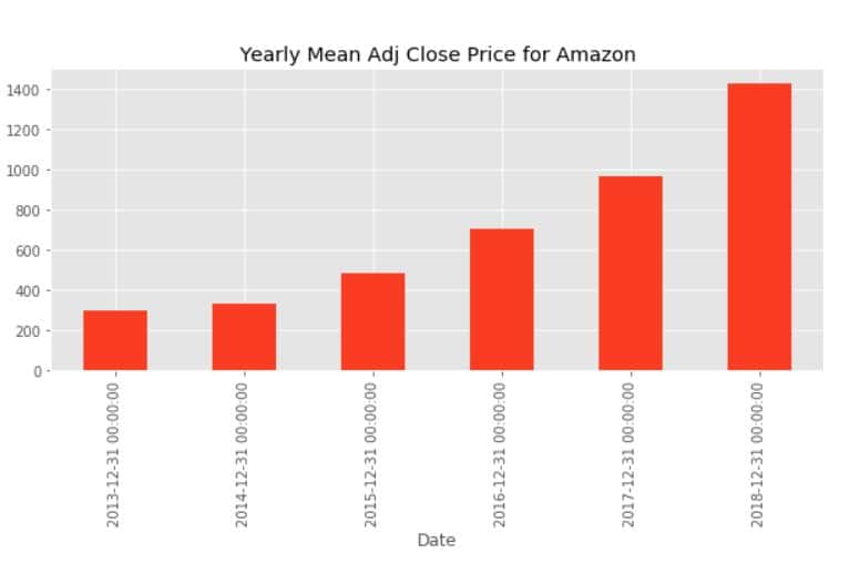
The above bar plot corresponds to Amazon’s average adjusted closing price at year-end for each year in our data set.
Similarly, monthly maximum opening price for each year can be found below.

Monthly maximum opening price for Amazon
Time shifting
Sometimes, we may need to shift or move the data forward or backwards in time. This shifting is done along a time index by the desired number of time-frequency increments.
...continue with Time Shifting and see the code in the Kite Github repo.
Parul Pandey is a Data Science Evangelist at H2O.ai and author for the Kite Blog.

Top comments (1)
The offset alias table is a good touch. Those are so hard to remember after not touching them for awhile, or dealing with odd ones. They also apply to the rolling method 😉.