Understanding Array Shapes in NumPy

Introduction

Numpy is a handy tool, which stands for Numerical Python, is super useful for doing math stuff with data. But let’s focus on one big idea: array shapes. Understanding array shapes is like knowing how the puzzle fits together – it’s important so that everything works smoothly. Just like you can’t put together puzzles with different numbers of pieces, you can’t do certain things if arrays don’t have the right shapes.

Why do these shapes matter? Well, they help us change how data looks for making pictures, combine info in cool ways, and do specific math things. Knowing about array shapes makes it easier to move around and work with data.

In this article, we’re going to dive into why array shapes are important. Let’s start exploring.

Basics of Array Shapes

Data analysis often requires handling vast amounts of information, and it’s crucial to understand how this data is organized. Enter the world of array shapes in NumPy. Think of array shapes as a way of arranging and understanding your data, much like organizing books on different shelves based on their sizes or genres.

One-dimensional Array

A one-dimensional array is the simplest form. It’s like a single line of data, similar to a row of books on a shelf. Each book (or piece of data) is called an “element”.

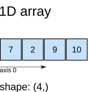
import numpy as np
one_dim_array = np.array([7, 2, 9, 10])

This gives us a line of numbers, starting from 7 and ending at 10.

Two-dimensional Array

Imagine stacking multiple rows of books one above the other; each row is like a one-dimensional array, but now we’ve added another dimension – the columns!

two_dim_array = np.array([[5.2, 3, 4.5], [9.1, 0.1, 0,3]])

Here, we have two rows and three columns, forming a 2×3 grid of numbers.

Three-dimensional Array

For a three-dimensional array, imagine a bookshelf where you have multiple sections, each with its own set of rows and columns of books. This is like having multiple matrices stacked behind one another.

three_dim_array = np.array([
    [[9, 6, 9], [1, 3, 0], [2, 9, 7], [1, 4, 7]], 
    [[9, 6, 8], [1, 3, 2], [2, 9, 5], [2, 3, 4]]
])

In this example, we’ve got two “sections” (or matrices). Each section has four rows and three columns of numbers.

Higher-dimensional Arrays

NumPy isn’t just limited to one, two, or three dimensions. It’s incredibly versatile and can handle even more complex structures. As you move into advanced data analysis, you might encounter situations where such multidimensional arrays come into play. For now, just remember that with NumPy, the sky is the limit!

higher_dim_array = np.array([
    [
        [[1, 2], [3, 4]], 
        [[5, 6], [7, 8]]
    ], 
    [
        [[9, 10], [11, 12]], 
        [[13, 14], [15, 16]]
    ]
])

Key Attributes of NumPy Arrays

Let’s take a moment to focus on some vital attributes that help describe our data’s organization. NumPy arrays have characteristics that give us insight into their structure: shape, ndim, and size.

Shape (shape)

The shape attribute provides a tuple representing the dimensionality of the array. It’s like measuring how many rows of books we have and how many books are in each row.

import numpy as np
data = np.array([[1, 2, 3], [4, 5, 6]])
print(data.shape) # (2, 3)

This tells us that our array has 2 rows and 3 columns.

Number of Dimensions (ndim)

The ndim attribute gives us the number of array dimensions or axes. Think of it as counting how many ways we can navigate through our collection of data.

import numpy as np
data = np.array([[1, 2, 3], [4, 5, 6]])
print(data.ndim) # 2

This confirms that our data has two dimensions, which makes sense as we saw with our shape example.

Size (size)
The size attribute tells us the total number of elements in the array. Imagine counting every single book on a large bookshelf, regardless of the row or section it’s in.

import numpy as np
data = np.array([[1, 2, 3], [4, 5, 6]])
print(data.size) # 6

This indicates there are 6 elements in total in our array, again aligning with our previous understanding.

Reshaping and Manipulating Array Shapes

Think of reshaping as rearranging puzzle pieces. Even though the pieces are the same, they can be organized differently to create unique pictures.

reshape Method

reshape allows us to change the structure of our array without changing the data itself.

import numpy as np
original_array = np.array([[2, 3, 4], [5, 6, 7]])
reshaped_array = original_array.reshape(3, 2)
print(reshaped_array)

# Output
[[2 3]
 [4 5]
 [6 7]]

Notice how the 2×3 grid transferred into a 3×2 grid, while the numbers themselves remained the same!

The Magic Number: -1 in Reshaping

Sometimes, we might want to reshape an array but let NumPy decide one of the dimensions for us. This is where the special value -1 comes in. When used in the reshape method, -1 basically tells NumPy: “Hey, I’m not sure about this dimension, can you figure it out for me?“

import numpy as np
original_array = np.array([1, 2, 3, 4, 5, 6])
reshaped_with_negative = original_array.reshape(3, -1)
print(reshaped_with_negative)

# Output
[[1 2]
 [3 4]
 [5 6]]

Here, we specified that we wanted 3 rows, but left the number of columns to NumPy’s discretion by using -1.

Flattening and Transposing Arrays

Let’s discuss two more powerful features that can make our data exploration even more interesting concepts: flattening and transposing arrays.

Flattening Arrays

Flattening, as the name suggests, is the process of converting a multi-dimensional array into a one-dimensional array. In NumPy, we’ve got two handy methods to achieve this: ravel() and flatten()

ravel() Method

This method provides a flattened array. However, it gives a “view” of the original array whenever possible. This means if you change the flat array, the original might change too.

import numpy as np

multi_dim_array = np.array([[1, 2, 3], [4, 5, 6]])
flat_using_ravel = multi_dim_array.ravel()

print(flat_using_ravel) # [1 2 3 4 5 6]

Now, let’s see how ravel() change the original data

import numpy as np

# Creating a 2x3 array
array_1 = np.array([[1, 2, 3], [4, 5, 6]])

# Using ravel() to flatten the array
raveled_array = array_1.ravel()

# Let's modify the flattened array
raveled_array[0] = 100

# Display the modified flattened array
print("Modified raveled array:", raveled_array)

# Now, let's check the original array
print("Original array after modification:", array_1)

# Output
Modified raveled array: [100   2   3   4   5   6]
Original array after modification: [[100   2   3]
                                    [  4   5   6]]

As you can see, changing the flattened array returned by ravel() also changes the original array.

flatten() Method

Unlike ravel(), the flatten() method always returns a fresh copy of the data. So, if you modify this flat version, the original stays the same.

import numpy as np
multi_dim_array = np.array([[1, 2, 3], [4, 5, 6]])
flat_using_flatten = multi_dim_array.flatten()
print(flat_using_flatten) # [1 2 3 4 5 6]

Now, let’s see how flatten() not change the original data

# Resetting our original array
array_1 = np.array([[1, 2, 3], [4, 5, 6]])

# Using flatten() to get a flattened array
flattened_array = array_1.flatten()

# Modifying the flattened array
flattened_array[0] = 100

# Display the modified flattened array
print("Modified flattened array:", flattened_array)

# Checking the original array
print("Original array after modification:", array_1)

# Output
Modified flattened array: [100   2   3   4   5   6]
Original array after modification: [[1 2 3]
                                    [4 5 6]]

Notice that even after modifying the array returned by flatten(), the original array remains unchanged.

Changing Directions with T: Transposing Arrays

The transposition of an array is like flipping its content over its diagonal. Rows become columns, and columns become rows. With NumPy, this magical switch is achieved with the T attribute.

import numpy as np
multi_dim_array = np.array([[1, 2, 3], [4, 5, 6]])
transposed_array = multi_dim_array.T
print(transposed_array)

# Output
[[1 4]
 [2 5]
 [3 6]]

Notice how our original 2×3 array has transformed into a 3×2 array!

Further Reading

• W3Schools; NumPy Array Shape
• A Comprehensive Guide to NumPy Arrays
• Understanding Array Broadcasting in NumPy
• Masking and Boolean Indexing: A Smart Data Filtering in Python
• A Beginner Guide to Data Manipulation in Python

Conclusion

In conclusion, understanding shapes in NumPy is like knowing how to build with blocks. It helps you work better with data. But just reading won’t make you an expert. You need to try it yourself, play with it, and learn from any mistakes. Keep practicing and trying new things in NumPy. Soon, you’ll get good at it. Happy coding!

---

👉 Visit my blog 👈