
The development of Keras started in early 2015. As of today, it has evolved into one of the most popular and widely used libraries built on top of Theano and TensorFlow. One of its prominent features is that it has a very intuitive and user-friendly API, which allows us to implement neural networks in only a few lines of code.
Keras is also integrated into TensorFlow from version 1.1.0. It is part of the contrib module (which contains packages developed by contributors to TensorFlow and is considered experimental code).
In this tutorial we will look at this high-level TensorFlow API by walking through:
- The basics of feedforward neural networks
- Loading and preparing the popular MNIST dataset
- Building an image classifier
- Train a neural network and evaluate its accuracy
Let's get started!
This tutorial is adapted from Part 4 of Next Tech’s Python Machine Learning series, which takes you through machine learning and deep learning algorithms with Python from 0 to 100. It includes an in-browser sandboxed environment with all the necessary software and libraries pre-installed, and projects using public datasets. You can get started for free here!
Multilayer Perceptrons
Multilayer feedforward neural networks are a special type of fully connected network with multiple single neurons. They are also called Multilayer Perceptrons (MLP). The following figure illustrates the concept of an MLP consisting of three layers:

The MLP depicted in the preceding figure has one input layer, one hidden layer, and one output layer. The units in the hidden layer are fully connected to the input layer, and the output layer is fully connected to the hidden layer. If such a network has more than one hidden layer, we also call it a deep artificial neural network.
We can add an arbitrary number of hidden layers to the MLP to create deeper network architectures. Practically, we can think of the number of layers and units in a neural network as additional hyperparameters that we want to optimize for a given problem task.
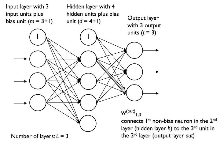
As shown in the preceding figure, we denote the ith activation unit in the ith layer as ai(l). To make the math and code implementations a bit more intuitive, we will use the in superscript for the input layer, the h superscript for the hidden layer, and the o superscript for the output layer.
For instance, ai(in) refers to the ith value in the input layer, ai(h) refers to the ith unit in the hidden layer, and ai(out) refers to the ith unit in the output layer. Here, the activation units a0(in) and a0(h) are the bias units, which we set equal to 1. The activation of the units in the input layer is just its input plus the bias unit:

Each unit in layer l is connected to all units in layer l + 1 via a weight coefficient. For example, the connection between the kth unit in layer l to the jth unit in layer l + 1 will be written as wk, j(l). Referring back to the previous figure, we denote the weight matrix that connects the input to the hidden layer as W(h), and we write the matrix that connects the hidden layer to the output layer as W(out).
We summarize the weights that connect the input and hidden layers by a matrix W(h) ∈ ℝ m × d, where d is the number of hidden units and m is the number of input units including the bias unit. Since it is important to internalize this notation to follow the concepts later in this lesson, let's summarize what we have just learned in a descriptive illustration of a simplified 3-4-3 multilayer perceptron:
The MNIST dataset
To see what neural network training via the tensorflow.keras (tf.keras) high-level API looks like, let's implement a multilayer perceptron to classify the handwritten digits from the popular Mixed National Institute of Standards and Technology (MNIST) dataset that serves as a popular benchmark dataset for machine learning algorithm.
To follow along with the code snippets in this tutorial, you can use this Next Tech sandbox, which has the MNIST dataset and all necessary packages installed. Otherwise, you can use your local environment and download the dataset here.
The MNIST dataset in four parts, as listed here:
-
Training set images:
train-images-idx3-ubyte.gz— 60,000 samples -
Training set labels:
train-labels-idx1-ubyte.gz— 60,000 labels -
Test set images:
t10k-images-idx3-ubyte.gz— 10,000 samples -
Test set labels:
t10k-labels-idx1-ubyte.gz— 10,000 labels
The training set consists of handwritten digits from 250 different people (50% high school students, 50% employees from the Census Bureau). The test set contains handwritten digits from different people.
Note that TensorFlow also provides the same dataset as follows:
import tensorflow as tf
from tensorflow.examples.tutorials.mnist import input_data
However, we work with the MNIST dataset as an external dataset to learn all the steps of data preprocessing separately. This way, you learn what you need to do with your own dataset.
The first step is to unzip the four parts of the MNIST dataset by running the following commands in your Terminal:
cd mnist/
gzip *ubyte.gz -d
Our images are stored in byte format, and we will read them into NumPy arrays that we will use to train and test our MLP implementation. In order to do that, we will define the following helper function:
import os
import struct

def load_mnist(path, kind='train'):
    """Load MNIST data from `path`"""
    labels_path = os.path.join(
        path, f'{kind}-labels-idx1-ubyte'
    )
    images_path = os.path.join(
        path, f'{kind}-images-idx3-ubyte'
    )

    with open(labels_path, 'rb') as lbpath:
        magic, n = struct.unpack('>II', lbpath.read(8))
        labels = np.fromfile(lbpath, dtype=np.uint8)

    with open(images_path, 'rb') as imgpath:
        magic, num, rows, cols = struct.unpack(">IIII", imgpath.read(16))
        images = np.fromfile(imgpath, dtype=np.uint8).reshape(len(labels), 784)
        images = ((images / 255.) - .5) * 2

    return images, labels
The load_mnist function returns two arrays, the first being an n x m dimensional NumPy array (images), where n is the number of samples and m is the number of features (here, pixels). The images in the MNIST dataset consist of 28 x 28 pixels, and each pixel is represented by a gray scale intensity value. Here, we unroll the 28 x 28 pixels into one-dimensional row vectors, which represent the rows in our images array (784 per row or image). The second array (labels) returned by the load_mnist function contains the corresponding target variable, the class labels (integers 0-9) of the handwritten digits.
Then, the dataset is loaded and prepared as follows:
# loading the data
X_train, y_train = load_mnist('./mnist/', kind='train')
print(f'Rows: {X_train.shape[0]},  Columns: {X_train.shape[1]}')

X_test, y_test = load_mnist('./mnist/', kind='t10k')
print(f'Rows: {X_test.shape[0]},  Columns: {X_test.shape[1]}')

# mean centering and normalization:
mean_vals = np.mean(X_train, axis=0)
std_val = np.std(X_train)

X_train_centered = (X_train - mean_vals)/std_val
X_test_centered = (X_test - mean_vals)/std_val

del X_train, X_test

print(X_train_centered.shape, y_train.shape)
print(X_test_centered.shape, y_test.shape)
[Out:]
Rows: 60000,  Columns: 784
Rows: 10000,  Columns: 784
(60000, 784) (60000,)
(10000, 784) (10000,)
To get an idea of how those images in MNIST look, let's visualize examples of the digits 0-9 via Matplotlib's imshowfunction:
import matplotlib.pyplot as plt

fig, ax = plt.subplots(nrows=2, ncols=5,
                       sharex=True, sharey=True)
ax = ax.flatten()
for i in range(10):
    img = X_train_centered[y_train == i][0].reshape(28, 28)
    ax[i].imshow(img, cmap='Greys')

ax[0].set_yticks([])
ax[0].set_xticks([])
plt.tight_layout()
plt.show()
We should now see a plot of the 2 x 5 subfigures showing a representative image of each unique digit:

Now let’s start building our model!
Building an MLP using TensorFlow's Keras API
First, let's set the random seed for NumPy and TensorFlow so that we get consistent results:
import tensorflow.contrib.keras as keras

np.random.seed(123)
tf.set_random_seed(123)
To continue with the preparation of the training data, we need to convert the class labels (integers 0-9) into the one-hot format. Fortunately, Keras provides a convenient tool for this:
y_train_onehot = keras.utils.to_categorical(y_train)

print('First 3 labels: ', y_train[:3])
print('\nFirst 3 labels (one-hot):\n', y_train_onehot[:3])
First 3 labels:  [5 0 4]

First 3 labels (one-hot):
 [[0. 0. 0. 0. 0. 1. 0. 0. 0. 0.]
 [1. 0. 0. 0. 0. 0. 0. 0. 0. 0.]
 [0. 0. 0. 0. 1. 0. 0. 0. 0. 0.]]
Now, let's implement our neural network! Briefly, we will have three layers, where the first two layers (the input and hidden layers) each have 50 units with the tanh activation function and the last layer (the output layer) has 10 layers for the 10 class labels and uses softmax to give the probability of each class. Keras makes these tasks very simple:
# initialize model
model = keras.models.Sequential()

# add input layer
model.add(keras.layers.Dense(
    units=50,
    input_dim=X_train_centered.shape[1],
    kernel_initializer='glorot_uniform',
    bias_initializer='zeros',
    activation='tanh')
)
# add hidden layer
model.add(
    keras.layers.Dense(
        units=50,
        input_dim=50,
        kernel_initializer='glorot_uniform',
        bias_initializer='zeros',
        activation='tanh')
    )
# add output layer
model.add(
    keras.layers.Dense(
        units=y_train_onehot.shape[1],
        input_dim=50,
        kernel_initializer='glorot_uniform',
        bias_initializer='zeros',
        activation='softmax')
    )

# define SGD optimizer
sgd_optimizer = keras.optimizers.SGD(
    lr=0.001, decay=1e-7, momentum=0.9
)
# compile model
model.compile(
    optimizer=sgd_optimizer,
    loss='categorical_crossentropy'
)
First, we initialize a new model using the Sequential class to implement a feedforward neural network. Then, we can add as many layers to it as we like. However, since the first layer that we add is the input layer, we have to make sure that the input_dim attribute matches the number of features (columns) in the training set (784 features or pixels in the neural network implementation).
Also, we have to make sure that the number of output units (units) and input units (input_dim) of two consecutive layers match. Our first two layers have 50 units plus one bias unit each. The number of units in the output layer should be equal to the number of unique class labels — the number of columns in the one-hot-encoded class label array.
Note that we used glorot_uniform to as the initialization algorithm for weight matrices. Glorot initialization is a more robust way of initialization for deep neural networks. The biases are initialized to zero, which is more common, and in fact the default setting in Keras.
Before we can compile our model, we also have to define an optimizer. We chose a stochastic gradient descent optimization. Furthermore, we can set values for the weight decay constant and momentum learning to adjust the learning rate at each epoch. Lastly, we set the cost (or loss) function to categorical_crossentropy.
The binary cross-entropy is just a technical term for the cost function in the logistic regression, and the categorical cross-entropy is its generalization for multiclass predictions via softmax).
After compiling the model, we can now train it by calling the fit method. Here, we are using mini-batch stochastic gradient with a batch size of 64 training samples per batch. We train the MLP over 50 epochs, and we can follow the optimization of the cost function during training by setting verbose=1.
The validation_split parameter is especially handy since it will reserve 10% of the training data (here, 6,000 samples) for validation after each epoch so that we can monitor whether the model is overfitting during training:
# train model
history = model.fit(
    X_train_centered, y_train_onehot,
    batch_size=64, epochs=50,
    verbose=1, validation_split=0.1
)
Printing the value of the cost function is extremely useful during training to quickly spot whether the cost is decreasing during training and stop the algorithm earlier. Otherwise, hyperparameter values will need to be tuned.
To predict the class labels, we can then use the predict_classes method to return the class labels directly as integers:
y_train_pred = model.predict_classes(X_train_centered, verbose=0)
print('First 3 predictions: ', y_train_pred[:3])
[Out:]
First 3 predictions: [5 0 4]
Finally, let's print the model accuracy on training and test sets:
# calculate training accuracy
y_train_pred = model.predict_classes(X_train_centered, verbose=0)
correct_preds = np.sum(y_train == y_train_pred, axis=0)
train_acc = correct_preds / y_train.shape[0]

print(f'Training accuracy: {(train_acc * 100):.2f}')

# calculate testing accuracy
y_test_pred = model.predict_classes(X_test_centered, verbose=0)
correct_preds = np.sum(y_test == y_test_pred, axis=0)
test_acc = correct_preds / y_test.shape[0]

print(f'Test accuracy: {(test_acc * 100):.2f}')
[Out:]
Training accuracy: 98.81
Test accuracy: 96.27
I hope you enjoyed this tutorial on using TensorFlow's keras API to build and train a multilayered neural network for image classification! Note that this is just a very simple neural network without optimized tuning parameters.
In practice you need to know how to optimize the model by tweaking learning rate, momentum, weight decay, and number of hidden units. You also need to learn how to deal with the vanishing gradient problem, wherein error gradients become increasingly small as more layers are added to a network.
We cover these topics in Next Tech's Python Machine Learning (Part 4) course, as well as:
- Breaking down the mechanics of
TensorFlow, such as tensors, activation functions computation graphs, variables, and placeholders - Low-level
TensorFlowand another high-level API,Layers - Modeling sequential data using recurrent neural networks (RNN) and long short-term memory (LSTM) networks
- Classifying images with deep convolutional neural networks (CNN).
You can get started here for free!

Top comments (0)