
This is a short continuation of my article on Data Structures and Algorithms in Python where I covered basic Data structures that a beginner in Python needs to know.
Here I will cover the Big O notation as an introduction to algorithms in Python. I will try to explain it in simple terms.
Big O notation is a mathematical notation that describes the limiting behavior of a function when the argument tends towards a particular value or infinity ~ Wikipedia
Big O notation is used to describe the performance of an algorithm.
It is used to classify algorithms according to how their run time or space requirements grow as the input size grows.
It helps us determine whether an algorithm is scalable or not, that is, is it going to scale well as the input grows really large?
Some operations can be more or less costly depending on the Data structure we use.
# example
given_list = [5, 1, 7, 2, 6, 3, 10, 4, 9]
def find_sum(given_list):
    total = 0
    for x in given_list:
        total += 1
    return total
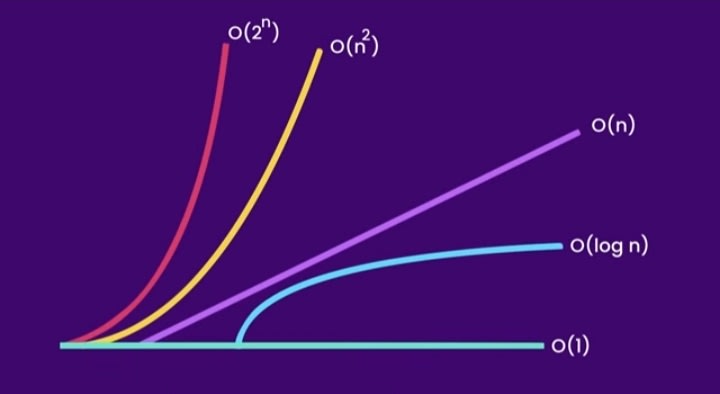
Examples of common growth rates/time complexities
Runtime is the time taken to execute a piece of code.
Time complexity is a way of showing how the runtime of a function increases as the size of input increases.
1.O(n)
Linear time complexity.
n - size of the input
In our example n is the number of elements in our list.
Simple loops run in linear time or O(n)
Here the cost of the algorithm increases linearly as the size of the input increases.
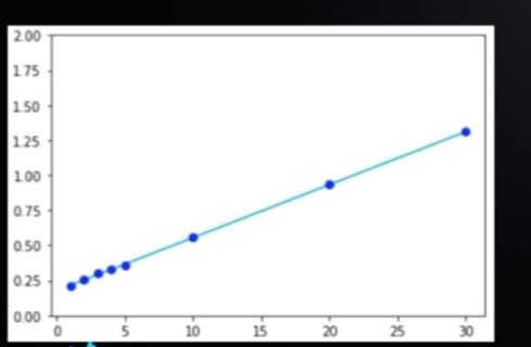
The time(T) it takes to run a function can be expressed as a linear function:
T = an + b
where T - time, a,b - constants, n - size of input
Steps to find which type of time complexity we are using
Find the fastest growing term in the given function.
Take out the coefficient out of the fastest growing term
What remains is what goes inside the brackets in our notation O(**).
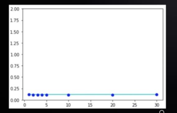
2.O(1)
(1) - refers to the run time complexity of the method.
Constant amount of time. This is when the amount of time it takes to complete a function does not increase as the size of input increases.
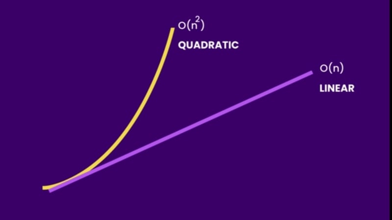
3.O(n^2)
Quadratic time complexity.
This is when the time taken to complete a function increases in quadratic form.
Nested loops run in quadratic time or O(n^2).
Algorithms that run in O(n^2) get slower than algorithms that run in O(n). As the input grows larger, algorithms that run in quadratic time get slower.
4.O(log n)
Logarithmic time
An algorithm with logarithmic time is more scalable than one with linear time.
Examples of algorithms that run in logarithmic time
Binary search

5.O(2^n)
Exponential time
Space complexity
Space complexity is the additional space that we should allocate relative to the size of the input.

Top comments (0)