A beginner’s guide to sentiment analysis using OceanBase and spaCy

In the modern commercial world, understanding your customer's sentiments is crucial. Businesses are progressively recognizing the importance of this aspect, as it allows them to gauge customer satisfaction, measure product reception, and understand market trends. This is where the power of Natural Language Processing (NLP) comes in, specifically through sentiment analysis.

Sentiment analysis, or opinion mining, uses NLP, text analysis, and computational linguistics to identify and extract subjective information from source materials. It's a method used to determine the attitudes, opinions, and emotions of a speaker or writer concerning some topic or the overall contextual polarity of a document.

In this article, I'm going to walk through a sentiment analysis project from start to finish, using open-source Amazon product reviews. However, using the same approach, you can easily implement mass sentiment analysis on your own products. We'll explore an approach to sentiment analysis with one of the most popular Python NLP packages: spaCy.

For the core database of my sentiment analysis projects, I'll be using OceanBase. OceanBase is a reliable and high-performance relational database that is well-suited for data scientists working on NLP projects. Its high scalability means it can handle the large amounts of data that are often a part of NLP projects.

Additionally, its capacity for high concurrency allows for multiple processes to be executed simultaneously, a beneficial feature when dealing with the complex computations required in NLP. Lastly, OceanBase's strong consistency ensures the integrity and accuracy of the data, a critical factor in any data analysis.

Setting up the environment

In this project, we’ll use Google Colab to run the sentiment analysis. I have included a Colab notebook that contains all the code and results of this project.

We start by importing the necessary Python libraries, including pandas for data manipulation, numpy for numerical computations, matplotlib and seaborn for data visualization, spaCy for natural language processing, and TextBlob for sentiment analysis.

import pandas as pd
import numpy as np
import matplotlib.pyplot as plt
import seaborn as sns
import spacy
from textblob import TextBlob

plt.style.use('ggplot')

To use OceanBase in the project, you first need a running OceanBase cluster. You have several options for doing so. You can install OceanBase in your local environment, spin up a virtual machine in the cloud to run it, or use OceanBase Cloud in the AWS marketplace to set up your cluster in just a few clicks. After setting up your OceanBase server, don’t forget to obtain the username, password, hostname, and port for later use.

Next, we set up our connection to OceanBase, a distributed relational database that is highly available and scalable. We use SQLAlchemy to create a connection with the database.

from sqlalchemy import create_engine
engine = create_engine('mysql+pymysql://username:password@hostname:2881/db')

We then create a table in OceanBase to store the reviews. The table includes columns for the product ID, user ID, profile name, helpfulness numerator and denominator, score, time, summary, and text of the review.

Explore the raw data

The raw data we are going to analyze comes from Kaggle, which is an online community of data scientists and machine learning practitioners. The open dataset consists of reviews of fine foods from Amazon. The data span a period of more than 10 years, including around 500,000 reviews up to October 2012. Reviews include product and user information, ratings, and a plain text review.

After loading our data into a data frame, we explore it by checking its shape and the first few rows. We also visualize the distribution of review scores.

df = pd.read_csv('path/to/file.csv')
print(df.shape)

And we see the following results

(568454, 10)

We can see that the original dataset contains nearly half a million reviews. A quick df.head() command will give us a preview of the dataset

Next, we visualize the distribution of review scores. This gives us an overview of the reviews. For instance, if most reviews have a score of 5, we can infer that customers are generally satisfied with the products.

ax = df['Score'].value_counts().sort_index() \
    .plot(kind='bar',
          title='Count of Reviews by Stars',
          figsize=(10, 5))
ax.set_xlabel('Review Stars')
plt.show()

Now we can upload the data frame, which contains all the reviews to the Reviews table in our OceanBase database.

# Upload the data frame to the OceanBase table
df.to_sql('Reviews', con=engine, if_exists='append', index=False)

Setting up s**entiment analysis functions**

Now, let's move on to the core part of our project - sentiment analysis. We start by loading the English model from spaCy.

# Load the nlp model
nlp = spacy.load('en_core_web_sm')

We define a function get_sentiment to calculate the sentiment polarity and subjectivity of a text. The polarity score ranges from -1 to 1 (where 1 is positive sentiment, -1 is negative sentiment, and 0 is neutral sentiment), and the subjectivity score ranges from 0 to 1 (where 0 is objective and 1 is subjective).

def get_sentiment(text):
    """This function receives a text and returns its sentiment polarity and subjectivity."""
    doc = nlp(text)
    sentiment = TextBlob(text).sentiment
    return sentiment

We test our function on a sample review from our dataset to make sure it's working as expected. Then, we apply this function to all reviews in our dataset and add new columns for polarity, subjectivity, and sentiment.

# Test the function on an example review
example = df['Text'][30]
print(example)
# I have never been a huge coffee fan. However, my mother purchased this little machine and talked me into trying the Latte Macciato. No Coffee Shop has a better one and I like most of the other products, too (as a usually non-coffee drinker!).<br />The little Dolche Guesto Machine is super easy to use and prepares a really good Coffee/Latte/Cappuccino/etc in less than a minute (if water is heated up). I would recommend the Dolce Gusto to anyone. Too good for the price and I'am getting one myself! :)

This gives us the following result:

get_sentiment(example)
# Sentiment(polarity=0.2557692307692308, subjectivity=0.5608974358974359)

This means that the sentiment of this review is positive and has a subjectivity score of around 0.56. Which is pretty accurate by telling from our human instincts.

In sentiment analysis, polarity determines the emotional state expressed in the text. The polarity score ranges from -1 to 1. A score closer to 1 means a higher degree of positivity, and a score closer to -1 means a higher degree of negativity.

Subjectivity, on the other hand, determines if the text is objective or subjective. The subjectivity score ranges from 0 to 1. A score closer to 0 is more objective, and a score closer to 1 is more subjective.

With the sentiment analysis function ready, we can run sentiment analysis against every row in our OceanBase database and store their sentiment and subjectivity in separate columns for future uses.

#### Run sentiment analysis in the reviews table
connection = engine.connect()

# Read the Reviews table into DataFrame
df = pd.read_sql_table('Reviews', connection)

# Apply the sentiment analysis function to the 'Text' column
df['Polarity'], df['Subjectivity'] = zip(*df['Text'].map(get_sentiment))
df['Sentiment'] = df['Polarity'].apply(lambda polarity : 'Positive' if polarity > 0 else 'Negative' if polarity < 0 else 'Neutral')
connection.close()

Now let’s take a look at the data frame

df.head()

We now have 3 new columns that represent the polarity, subjectivity, and sentiment of each review.

To preserve the original raw data, I will store the new data frame in a separate table in OceanBase

# Write the DataFrame back to OceanBase and store it in the 'Sentiment' table
connection = engine.connect()
df.to_sql('Sentiment', con=engine, if_exists='replace', index=False)
connection.close()

Sentiment analysis of the data

In this section, I will try to go through some of the most popular sentiment analysis paradigms of product reviews using data stored in our OceanBase database, then we will try to do some sophisticated analyses to demonstrate the power of NLP and how it can be used in business intelligence.

Sentiment distribution - an overview

First, we read the Sentiment table into a data frame and separate the data based on sentiment. We then visualize the score distribution for each sentiment using histograms. This allows us to see if there is a relationship between the sentiment of a review and the score it gives.

# Count the number of positive, negative and neutral reviews
sentiment_counts = df['Sentiment'].value_counts()
print(sentiment_counts)

# Visualize the sentiment distribution
plt.figure(figsize=(10,5))
sns.barplot(x=sentiment_counts.index, y=sentiment_counts.values, alpha=0.8)
plt.title('Sentiment Distribution')
plt.ylabel('Number of Occurrences', fontsize=12)
plt.xlabel('Sentiment', fontsize=12)
plt.show()

#### We are expected to see the following results:
# Positive    881
# Negative     98
# Neutral      21
# Name: Sentiment, dtype: int64

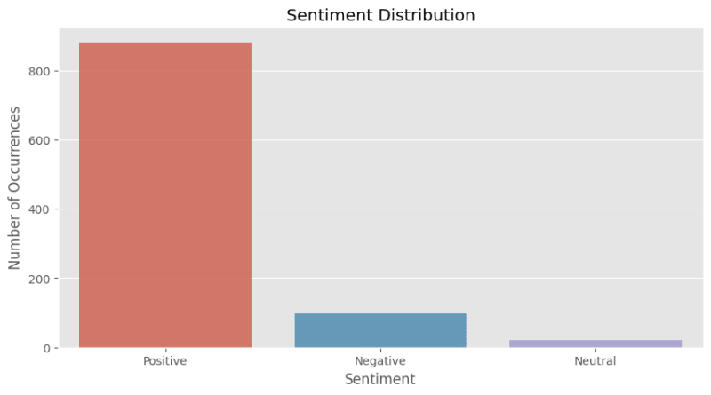
From this overview, we can tell that most of the reviews are positive.

Understanding Score Distribution by Sentiment

Now let’s try to visualize the score distribution for positive, negative, and neutral reviews. It separates reviews based on their sentiment and plots a histogram for each sentiment to show the distribution of scores.

This analysis can provide valuable insights for businesses. For example, if a business notices that the majority of positive reviews are scoring a 4 instead of a 5, they might investigate what is preventing customers from giving a perfect score.

# Separate the data based on sentiment
positive_reviews = df[df['Sentiment'] == 'Positive']
negative_reviews = df[df['Sentiment'] == 'Negative']
neutral_reviews = df[df['Sentiment'] == 'Neutral'] # Assuming you have neutral reviews

# Plotting
fig, axs = plt.subplots(3, figsize=(10, 15))

# Positive reviews
axs[0].hist(positive_reviews['Score'], bins=5, color='green', edgecolor='black')
axs[0].set_title('Score Distribution for Positive Reviews')
axs[0].set_xlabel('Score')
axs[0].set_ylabel('Frequency')

# Negative reviews
axs[1].hist(negative_reviews['Score'], bins=5, color='red', edgecolor='black')
axs[1].set_title('Score Distribution for Negative Reviews')
axs[1].set_xlabel('Score')
axs[1].set_ylabel('Frequency')

# Neutral reviews
axs[2].hist(neutral_reviews['Score'], bins=5, color='blue', edgecolor='black')
axs[2].set_title('Score Distribution for Neutral Reviews')
axs[2].set_xlabel('Score')
axs[2].set_ylabel('Frequency')

plt.tight_layout()
plt.show()

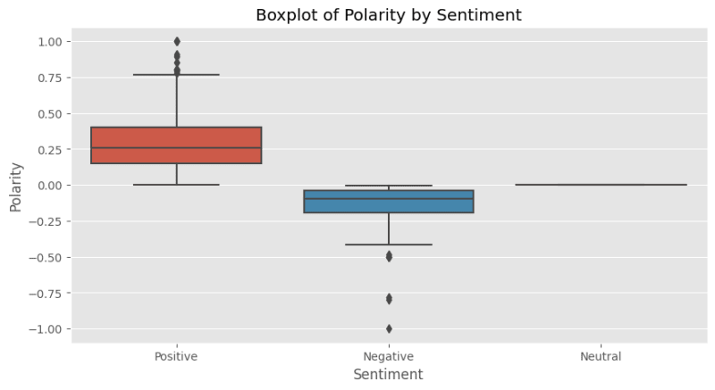
Boxplot of polarity by sentiment

We use a boxplot to visualize the distribution of polarity scores for each sentiment. This helps us understand the spread and skewness of the polarity scores. If the boxplot for a sentiment is skewed, it means that the reviews of that sentiment tend to be more positive or negative.

# Boxplot of Polarity by Sentiment
plt.figure(figsize=(10,5))
sns.boxplot(x='Sentiment', y='Polarity', data=df)
plt.title('Boxplot of Polarity by Sentiment')
plt.show()

Time Series Analysis

We analyze how sentiments and scores have evolved over time by converting the 'Time' column into a readable format and plotting a stacked bar plot of sentiment over time. This can help us identify trends and patterns in the sentiment of reviews over time.

# Time Series Analysis
# Convert 'Time' to datetime and extract the year
df['Time'] = pd.to_datetime(df['Time'], unit='s')
df['Year'] = df['Time'].dt.year

plt.figure(figsize=(10,5))
df.groupby(['Year', 'Sentiment']).size().unstack().plot(kind='bar', stacked=True)
plt.title('Sentiment Over Time')
plt.show()

Correlation Matrix

We can use a correlation matrix to understand the relationships between different numerical variables. This can help us identify if certain variables are associated with one another.

# Correlation Matrix
plt.figure(figsize=(10,5))
sns.heatmap(df[['HelpfulnessNumerator', 'HelpfulnessDenominator', 'Score', 'Polarity', 'Subjectivity']].corr(), annot=True, cmap='coolwarm')
plt.title('Correlation Matrix')
plt.show()

Word cloud of positive and negative reviews

Now, we can generate a word cloud for each sentiment to give us a visual representation of the most common words in positive, and negative reviews. This can help us understand the common themes in each sentiment.

from wordcloud import WordCloud

# Combine all reviews for the desired sentiment, remove 'br' (line breaks) from the text
positive_text = ' '.join(df[df['Sentiment']=='Positive']['Text'].tolist()).replace('br', '')
negative_text = ' '.join(df[df['Sentiment']=='Negative']['Text'].tolist()).replace('br', '')

# Generate word clouds
wordcloud_positive = WordCloud(background_color='white').generate(positive_text)
wordcloud_negative = WordCloud(background_color='white').generate(negative_text)

# Plot word clouds
plt.figure(figsize=(10, 5))

plt.subplot(1, 2, 1)
plt.imshow(wordcloud_positive, interpolation='bilinear')
plt.axis('off')
plt.title('Word Cloud of Positive Sentiment')

plt.subplot(1, 2, 2)
plt.imshow(wordcloud_negative, interpolation='bilinear')
plt.axis('off')
plt.title('Word Cloud of Negative Sentiment')

plt.show()

Like the opening of Leo Tolstoy's novel Anna Karenina: “Happy families are all alike; every unhappy family is unhappy in its own way,” there isn’t much to analyze in positive reviews, but in negative reviews, we can easily find out people were complaining about the taste and packing of the products. Remember, this dataset focuses on food reviews on Amazon.

Sentiment by Day of Week

Sometimes, people give reviews based on their mood. And people usually have better moods on weekends than on Mondays. We can analyze if there is any pattern in sentiment based on the day of the week the review was posted. This can help businesses understand if there are any temporal trends in customer sentiment.

# Sentiment by Day of Week

df['DayOfWeek'] = df['Time'].dt.dayofweek

df.groupby(['DayOfWeek', 'Sentiment']).size().unstack().plot(kind='bar', stacked=True)
plt.title('Sentiment by Day of Week')
plt.xlabel('Day of Week (0=Monday, 6=Sunday)')
plt.ylabel('Number of Reviews')
plt.show()

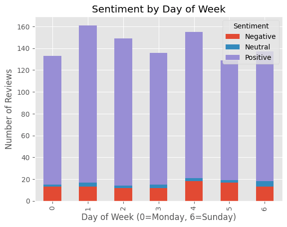
Well, it turned out the result somehow doesn’t reflect our hypothesis. But you can try it on your own dataset, and perhaps you will find something interesting.

Length of Review vs. Helpfulness

Now let’s try to see if there's a correlation between the length of the review and its helpfulness. This can provide insights into how much detail customers find useful in reviews.

# Calculate review length and filter the DataFrame
df['ReviewLength'] = df['Text'].apply(len)
df_filtered = df[(df['ReviewLength'] > 1) & (df['ReviewLength'] <= 2000)]

# Length of Review vs. Helpfulness
plt.figure(figsize=(10,5))
sns.scatterplot(x='ReviewLength', y='HelpfulnessNumerator', hue='Sentiment', data=df_filtered)
plt.title('Length of Review vs. Helpfulness')
plt.xlabel('Review Length')
plt.ylabel('Helpfulness')
plt.show()

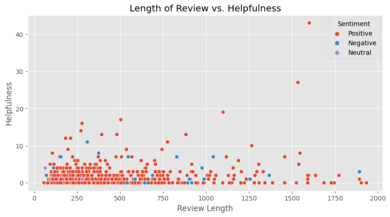
It turned out that lengthy reviews are not necessarily more helpful according to other users’ feedback. But some extremely long reviews, like this one with around 1,600 characters, did receive the highest score of helpfulness.

Correlation between Subjectivity and Score

We can also visualize the correlation between the subjectivity of a review and the score it gives. This can help us understand if more subjective or objective reviews tend to give higher or lower scores.

# Correlation between Subjectivity and Score
plt.figure(figsize=(10,5))
sns.scatterplot(x='Subjectivity', y='Score', hue='Sentiment', data=df)
plt.title('Correlation between Subjectivity and Score')
plt.xlabel('Subjectivity')
plt.ylabel('Score')
plt.show()

Find out the most beloved products

Identifying the most loved products is an essential aspect of running a successful e-commerce business. It provides sellers with valuable insights into customer preferences and product performance, which can be used to drive strategic decisions and business growth.

Understanding which products are most loved can help e-commerce sellers allocate their resources more effectively. This includes decisions about inventory management, marketing budget allocation, and even product development.

Here’s how you can do it with our Sentiment dataset stored in OceanBase:

from IPython.display import display

# Create a new DataFrame to count the number of reviews and average scores
grouped = df.groupby('ProductId').agg({'Score': ['count', 'mean']})

# Create a new DataFrame to count the number of positive reviews
positive_reviews = df[df['Sentiment'] == 'Positive'].groupby('ProductId').count()

# Add the positive reviews count to the grouped DataFrame
grouped['PositiveReviewsCount'] = positive_reviews['Sentiment']

# Sort the values by count and mean score both in descending order to get most reviewed and highest scored products.
grouped.sort_values(by=[('Score', 'count'), ('Score', 'mean'), 'PositiveReviewsCount'], ascending=[False, False, False], inplace=True)

# Take the top 10
top_10 = grouped.head(10)

# Use Styler to add some background gradient
styled = top_10.style.background_gradient()

# Display the styled DataFrame
display(styled)

And we get this chart which gives us the top 10 “most beloved” products depending on their number of positive reviews and overall score.

The performance of a product is not just about sales numbers; customer reviews and sentiments are a significant part of this equation. A product might be a best-seller, but if the majority of reviews are negative, it might indicate a problem with the product that needs to be addressed. In this data set, we can easily find that product “B000HDMUQ2" is popular but received a mediocre review.

Conclusion

Sentiment analysis is a powerful tool that can provide profound insights into customer preferences and behaviors. By analyzing these Amazon reviews, we can understand not only the polarity of sentiments but also the subjectivity of the reviews. This analysis can shed light on the emotional state and personal biases of the reviewers.

While this particular sentiment analysis project focused on Amazon reviews as an example, the methodologies and tools employed here can be applied to much more complex and diverse datasets. For instance, you could analyze social media posts to understand public sentiment about a particular topic or event, customer support transcripts to discover common issues and pain points, or even news articles to identify trends and biases in media coverage.

And of course, having a robust, scalable, and reliable database is essential for any data scientist working on large-scale projects. The ability to handle vast amounts of data efficiently and conduct complex computations quickly is crucial for timely and accurate analysis. I think this is where OceanBase shines.

Sentiment analysis using NLP and OceanBase can provide data scientists with invaluable insights that can guide their strategies, improve their services, and ultimately increase customer satisfaction.

By harnessing these tools, data scientists can gain a deeper understanding of the sentiments in unstructured text data, enabling them to obtain insights that will lead to better decisions and improved products and services.

I've included all the code and results from this sentiment analysis project in a Google Colab notebook. It's a comprehensive resource that walks you through each step of the analysis, from setting up the environment to visualizing the results.

I encourage you to copy the notebook and experiment with it. Feel free to modify the code, try different parameters, or even apply the methodology to your own datasets. It's a great way to learn more about sentiment analysis, natural language processing, and the capabilities of OceanBase. You're welcome to use it as a starting point for your own data analysis projects.