In the modern landscape of data management and processing, the need for sophisticated data models and methodologies that can handle complex data structures has never been more imperative. The advent of graph data, with its unique ability to represent intricate relationships naturally and intuitively, has opened up a new frontier in data analysis.
While established graph databases like Neo4j offer robust solutions for handling graph data, the idea of integrating graph data into SQL databases offers potential advantages worth exploring. SQL databases are well-regarded for their ability to handle structured data efficiently, offering robustness, reliability, and a familiar query language (SQL). In this article, I will try to explore the potential implementation of graph data and graph queries in OceanBase, an open-source distributed SQL database.
By harnessing the power of graph data within a SQL database, we aim to combine the strengths of both paradigms - the structured data handling of SQL databases with the flexible, relationship-focused nature of graph data.
This article is an initial exploration of the potential benefits, challenges, and implications of incorporating graph data into the OceanBase ecosystem. I’ll dive into the reasons behind this integration, explore potential data modeling strategies, and discuss some sample queries. We'll also critically evaluate the performance implications and the limitations that could arise during this implementation.
My aim is not to provide a definitive solution but to stimulate a conversation and inspire further research on this topic. The final section of the article will offer some suggestions for the OceanBase team, hoping to contribute to the ongoing evolution of the database.
What is graph data and why it is important
Graph data is a form of data that captures entities, known as nodes or vertices, and the relationships between these entities, known as edges or links. This flexible structure enables graph data to model intricate relationships and complex systems with a high degree of fidelity, making it a powerful tool in diverse fields, from social network analysis to supply chain management.
Graph data is characterized by its non-linearity and the absence of a predetermined schema, which distinguishes it from traditional relational databases. The focus is not on the data itself but on the relationships between the data. This relationship-centric approach allows for deep, multi-layered analysis and can reveal insights that may remain hidden in more traditional data structures.
To illustrate, consider a social media platform. In this context, individual users can be represented as nodes, and the connections between them - friendships, messages, interactions - can be represented as edges.

A graph data model would allow us to map out the entire network, providing a detailed picture of how users interact with each other. This could reveal patterns and insights such as the most influential users, communities within the larger network, and potential pathways for information flow.
Why OceanBase users should care about graph data?
The idea to explore the integration of graph data into OceanBase is driven by the increasing prevalence of mixed data models in modern applications. As businesses and organizations tackle more complex problems and seek to extract more value from their data, they often find themselves needing to combine the structured, tabular data model offered by SQL databases with graph data. Since I have developed multiple projects based on OceanBase, it is an ideal platform for me to do such an experiment.
Numerous potential use cases could benefit from this integration. For example, in online finance and recommendation systems, the ability to efficiently trace and analyze connections could prove invaluable. In other words, by trying to implement graph data in OceanBase, we're not only trying to enrich its capabilities but also expand its potential applications.
However, challenges exist. The unique nature of graph data, with its focus on relationships over individual data points, presents new problems in terms of data modeling, query language, and performance optimization. The following sections will dive into these issues, providing a comprehensive analysis of the feasibility and potential benefits of this integration.
Modeling of graph data in OceanBase
To model graph data within OceanBase, we would essentially be creating a relational representation of our graph. The graph is broken down into its fundamental components: vertices (or nodes) and edges (or relationships). This approach is commonly known as the adjacency list model.
The adjacency list model involves two tables: one for vertices and one for edges. The Vertices table stores information about each vertex, while the Edges table stores information about each edge, including the vertices it connects.
Let's look at how these tables can be structured in OceanBase:
Create the vertex table:
CREATE TABLE Vertices (
    VertexID INT PRIMARY KEY,
    VertexProperties JSON
);
In this table, VertexID is the primary key that uniquely identifies each vertex. VertexProperties is a JSON field that stores the properties of each vertex. This structure allows us to represent a wide range of data types and complexities.
The edge table schema:
CREATE TABLE Edges (
    EdgeID INT PRIMARY KEY,
    SourceVertexID INT,
    TargetVertexID INT,
    EdgeProperties JSON,
    FOREIGN KEY (SourceVertexID) REFERENCES Vertices(VertexID),
    FOREIGN KEY (TargetVertexID) REFERENCES Vertices(VertexID)
);
In the Edges table, EdgeID is the primary key that uniquely identifies each edge. SourceVertexID and TargetVertexID identify the vertices that this edge connects, and EdgeProperties is a JSON field that stores the properties of each edge. The FOREIGN KEY constraints ensure that every edge corresponds to valid vertices in the Vertices table.
With the schemata of each table set, let’s try to create some dummy data in the database for later queries.
In the Vertices table, I will try to create 1,000 rows that represent users in an online transaction app.
CREATE FUNCTION random_ip() RETURNS TEXT DETERMINISTIC
BEGIN
  RETURN CONCAT(
    FLOOR(RAND() * 255) + 1, '.',
    FLOOR(RAND() * 255) + 0, '.',
    FLOOR(RAND() * 255) + 0, '.',
    FLOOR(RAND() * 255) + 0
  );
END;

CREATE FUNCTION random_device() RETURNS TEXT DETERMINISTIC
BEGIN
  DECLARE device TEXT;
  SET device = CASE FLOOR(RAND() * 6)
    WHEN 0 THEN 'IPHONE'
    WHEN 1 THEN 'ANDROID'
    WHEN 2 THEN 'PC'
    WHEN 3 THEN 'IPAD'
    WHEN 4 THEN 'TABLET'
    ELSE 'LAPTOP'
  END;
  RETURN device;
END;

CREATE PROCEDURE InsertRandomUsers()
BEGIN
  DECLARE i INT DEFAULT 0;
  WHILE i < 1000 DO
    INSERT INTO Vertices (VertexID, VertexProperties)
    VALUES (i+1, CONCAT(
      '{"name": "User', i+1,
      '", "email": "user', i+1,
      '@email.com", "ip":"', random_ip(),
      '", "DEVICE": "', random_device(), '"}'
    ));
    SET i = i + 1;
  END WHILE;
END;

CALL InsertRandomUsers();
The “users” in the table have properties such as IP, device, and email. With this setup, it is possible to explore how to implement anti-money laundry and fraud detection algorithms in an online transaction app. However, the situation in the real world will be much more complicated, thus these nodes will have more properties for analysis.
Now, let’s try to create some dummy data for the Edges table, with each row representing a “transaction” between each “user.” Each transaction will only have one property-the amount of the transaction.
-- Create a temporary table to hold a series of numbers
CREATE TEMPORARY TABLE temp_numbers (
    number INT
);

-- Stored procedure to fill the temporary table
DELIMITER //
CREATE PROCEDURE FillNumbers(IN max_number INT)
BEGIN
  DECLARE i INT DEFAULT 1;
  WHILE i <= max_number DO
    INSERT INTO temp_numbers VALUES (i);
    SET i = i + 1;
  END WHILE;
END //
DELIMITER ;

-- Call the procedure again to fill the temporary table with numbers from 1 to 1000
CALL FillNumbers(10000);

-- Use the temporary table to insert 1000 edges
INSERT INTO Edges (EdgeID, SourceVertexID, TargetVertexID, EdgeProperties)
SELECT
  number,
  FLOOR(1 + RAND() * 1000),
  FLOOR(1 + RAND() * 1000),
  CONCAT('{"amount": ', FLOOR(10 + RAND() * 1000), ', "date": "', DATE(NOW() - INTERVAL FLOOR(1 + RAND() * 365) DAY), '"}')
FROM temp_numbers;
This SQL query will create 10,000 random transactions in the Edges table. The data will also indicate the sender(SourceVertexID) and receiver(TargetVertexID) of the transaction.
Now here is what our database looks like.
Vertices:

Edges:

This example demonstrates a basic way to model graph data in OceanBase. It shows that even without native graph support, it's possible to implement graph-like structures in OceanBase. However, this approach has its limitations, especially when it comes to complex graph operations and performance, which we will discuss in the subsequent sections.
Some sample queries
Building on the adjacency list model we have implemented in OceanBase, we can now perform a variety of graph queries. In this section, I will try to run some sample queries using typical graph algorithms. It's worth noting that OceanBase's support for the recursive Common Table Expressions (CTEs) makes recursive queries possible, which is crucial for many graph algorithms.
Breadth-First Search (BFS)
Breadth-first search is a common algorithm used in graph data to find the shortest path from a starting node to a target node. It's particularly useful for exploring the connections between nodes in a graph. We can use recursive CTEs in OceanBase to implement BFS.
Suppose we want to find all users reachable within 3 steps (or transactions) from a specific user (with VertexID = 1), we can use the following query:
WITH RECURSIVE bfs AS (
    SELECT SourceVertexID, TargetVertexID, 1 AS depth
    FROM Edges
    WHERE SourceVertexID = 1
    UNION ALL
    SELECT Edges.SourceVertexID, Edges.TargetVertexID, bfs.depth + 1
    FROM Edges JOIN bfs ON Edges.SourceVertexID = bfs.TargetVertexID
    WHERE bfs.depth < 3
)
SELECT * FROM bfs;
In this query, the WITH RECURSIVE clause creates a recursive CTE named bfs. The CTE starts with all edges originating from the node with VertexID = 1. It then repeatedly adds edges that connect from the previously found nodes until it reaches a depth of 3.
The BFS query returns a set of all users that can be reached within 3 transactions from the user with VertexID = 1 (or other nodes based on your choice).
This result provides insights into the transaction network of the initial user, revealing users that are closely connected (within 3 transactions) to the initial user. This information can be useful in various applications such as fraud detection, where closely connected users may indicate suspicious activities.
In the query against my dummy database, I retrieved 871 rows of data with 131 ms. This is not too bad considering it contains 1,000 nodes and 10,000 edges.
Detecting Circular Transactions
Circular transactions, where money is transferred around a loop of accounts, can be a signal of fraudulent or money laundering activities. Identifying such loops can be a useful way to detect suspicious activity. We can use a depth-first search (DFS) algorithm to find such loops. Here is an example of how that might be done with a maximum path length of 5:
WITH RECURSIVE dfs AS (
    SELECT SourceVertexID, TargetVertexID, CAST(CONCAT(SourceVertexID, '-', TargetVertexID) AS CHAR(1000)) AS path, 1 AS depth
    FROM Edges
    WHERE SourceVertexID = 1
    UNION ALL
    SELECT dfs.SourceVertexID, Edges.TargetVertexID, CONCAT(dfs.path, '-', Edges.TargetVertexID), dfs.depth + 1
    FROM Edges JOIN dfs ON Edges.SourceVertexID = dfs.TargetVertexID
    WHERE dfs.depth < 5 AND dfs.SourceVertexID != Edges.TargetVertexID AND dfs.path NOT LIKE CONCAT('%-', Edges.TargetVertexID, '-%')
)
SELECT * FROM dfs WHERE SourceVertexID = TargetVertexID;
In this query, the WITH RECURSIVE clause creates a recursive CTE named dfs. The CTE starts with all edges originating from the node with VertexID = 1. It then repeatedly adds edges that connect from the previously found nodes until it reaches a depth of 5 or it finds a circular transaction (where SourceVertexID = TargetVertexID). The path column tracks the path taken by the DFS, which is used to ensure that the same node is not visited twice.
Identifying High-Frequency Transaction Pairs
In an online transaction system, if two users are frequently transacting with each other, it could indicate a strong relationship between them, or it could be a sign of suspicious activity. We can use a simple SQL query to find pairs of users who have transacted with each other more than a certain number of times:
SELECT SourceVertexID, TargetVertexID, COUNT(*) AS transaction_count
FROM Edges
GROUP BY SourceVertexID, TargetVertexID
HAVING transaction_count > 5
ORDER BY transaction_count DESC;
This query groups the transactions by the source and target vertices (i.e., the users involved in the transaction) and counts the number of transactions for each pair. It then filters out pairs with less than 5 transactions and orders the result by the number of transactions.
In this example, the algorithm took 127 milliseconds to complete querying all 10,000 transactions.
Uncovering Unusually Large Transactions
Sometimes, unusually large transactions may be a sign of potential fraud. We can use SQL to identify transactions where the amount is higher than a certain threshold (in this case, the threshold is set to 990 because the dummy data is random between 1 and 1,000. But you can set a more realistic threshold in your case).
Suppose we want to not only find transactions where the amount is higher than a certain threshold but also want to include information about the sender and recipient, such as their device, IP, and transaction date. We also want to order the results by the transaction amount and date. Here's how we can do that:
SELECT
    e.SourceVertexID,
    e.TargetVertexID,
    JSON_EXTRACT(e.EdgeProperties, '$.amount') AS transaction_amount,
    JSON_EXTRACT(e.EdgeProperties, '$.date') AS transaction_date,
    JSON_EXTRACT(s.VertexProperties, '$.DEVICE') AS sender_device,
    JSON_EXTRACT(s.VertexProperties, '$.ip') AS sender_ip,
    JSON_EXTRACT(r.VertexProperties, '$.DEVICE') AS recipient_device,
    JSON_EXTRACT(r.VertexProperties, '$.ip') AS recipient_ip
FROM
    Edges AS e
JOIN
    Vertices AS s ON e.SourceVertexID = s.VertexID
JOIN
    Vertices AS r ON e.TargetVertexID = r.VertexID
WHERE
    JSON_EXTRACT(e.EdgeProperties, '$.amount') > 990
ORDER BY
    transaction_amount DESC,
    transaction_date DESC;
In this query, we join the Edges table with the Vertices table twice - once for the sender (source vertex) and once for the recipient (target vertex). We then extract additional information about the sender and recipient from the VertexProperties field. Finally, we order the results by the transaction amount and date in descending order. This query gives us a more comprehensive view of large transactions, including who is involved and what devices they're using.

The performance of this query is influenced by the complexity of joining two tables and extracting JSON properties. While the query executed swiftly with smaller datasets, it will show a noticeable slowdown as the volume of data increases. Specifically, as the number of transactions (edges) and users (vertices) grew, the time taken to join tables and parse JSON properties increased, leading to longer execution times. Thus, although the query provided valuable insights, its scalability and performance on larger datasets could be a concern.
Performance
Based on the experiments, the performance of implementing graph data in OceanBase was a mixed bag. On the positive side, the adjacency list model was proven possible to implement, and basic graph operations, such as BFS and identifying high-frequency transaction pairs, ran efficiently. With a dataset of 1,000 nodes and 10,000 edges, these queries were executed in less than 200 milliseconds, which is more than satisfactory for a lot of real-world applications.
However, the performance of more complex graph operations, such as DFS, left much to be desired. The execution time of these operations grew exponentially with the depth or complexity of the operation, suggesting that the adjacency list model might not be scalable for large or complex graphs.
In the DFS example, when I set the depth to 5, the query was completed in 428 ms. However, increasing the depth to 6 caused the query time to surge to nearly 4.785 seconds, an approximately 11-fold increase. Further increasing the search depth to 7 resulted in the query taking an overwhelming 67.843 seconds to complete, marking a 14-fold increase from the previous depth. This pattern suggests an exponential growth in query time as the depth increases.
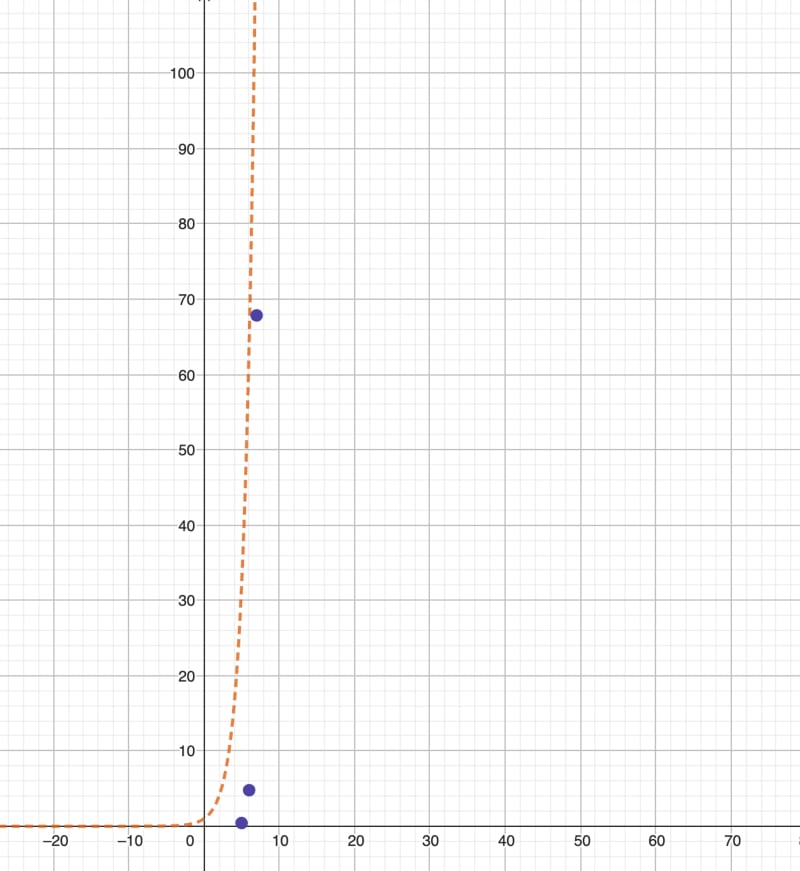
The query time for the DFS algorithm grows exponentially as the depth grows.
This performance degradation can be a significant barrier for real-time or near-real-time applications, where rapid responses are critical. Furthermore, large-scale graphs with thousands or millions of nodes and edges could exacerbate these performance issues, making the queries impractical for use in production databases.
Another performance issue was the overhead of JSON processing. While using JSON fields provided great flexibility in modeling graph data, it also added significant overhead to the database operations. Queries that involved multiple JSON extractions or manipulations were noticeably slower, and this overhead would likely increase with larger and more complex JSON objects.
The inherent limitations of SQL posed significant challenges for performing certain graph operations. For example, graph algorithms that required maintaining state across iterations, such as Dijkstra's algorithm, could not be implemented using SQL alone.
Interestingly, a 2019 study conducted by a team at Alibaba demonstrated the performance of relational databases in implementing graph data against a massive 10-billion-scale graph dataset. The research highlighted the efficiency of PostgreSQL's CTE syntax in implementing graph search requirements such as N-depth search, shortest path search, and controlling and displaying the tier depth.
In the context of a 5 billion point-edge network, N-depth searches and shortest path searches all had response times in “the millisecond range,” according to the Alibaba research. This is particularly notable when conducting a 3-depth search with a limit of 100 records per tier, where the response time was only 2.1 milliseconds, and the Transactions Per Second (TPS) reached 12,000. This impressive performance could serve as a benchmark for the OceanBase team in optimizing their graph data implementation.
Graph data in OceanBase: What’s next?
While OceanBase has made significant strides in providing robust, reliable, and scalable SQL database services, the integration of graph data handling capabilities could further enhance its value proposition. This article has demonstrated that basic graph data handling is indeed possible in OceanBase, but there are areas for improvement.
Here are some suggestions for the OceanBase team based on the discoveries made during this exploration:
- Optimize JOIN operations for graph data: Graph queries often involve complex JOIN operations. Optimizing these operations specifically for graph data could significantly improve performance. This could involve creating specialized indexes for graph data or implementing more efficient algorithms for JOIN operations.
- Improve JSON parsing performance: JSON parsing can be a significant bottleneck in graph queries. Techniques such as pre-parsing JSON fields, caching parsed results, or implementing more efficient JSON parsing algorithms could help improve performance.
- Implement graph-specific indexing: Indexing greatly improves query performance in SQL databases. Creating specialized indexes for graph data, such as indexes on edge properties or composite indexes on (source, target) vertex pairs, could make graph queries run faster.
This exploration into the incorporation of graph data into OceanBase has revealed a promising yet challenging road ahead. The potential to harness the power of graph data within the existing SQL structure offers exciting possibilities for expanding the range of applications and improving data analysis capabilities. However, the performance of complex graph operations and the processing overhead of JSON data present significant hurdles to overcome.
This exploration has only scratched the surface of what's possible, and there's much more to uncover. I hope that this article will stimulate further discussion, contributing to the ongoing evolution of OceanBase and similar databases.

Top comments (0)
Some comments may only be visible to logged-in visitors. Sign in to view all comments.