Statistics Cheatsheet – A Handy Guide for Enthusiasts

This cheatsheet provides a concise overview of key statistical concepts. While I’ve explained them through examples, having some prior knowledge will help you grasp them more effectively. That said, feel free to dive in, I hope you find it useful!

And a little shameless self-promotion – This blog is also here to introduce you to our YouTube learning platform, "Gistr", You can find the link at the end. If you're eager to learn through engaging video content, give it a try, you might find it incredibly helpful!

1. Counting & Combinatorics

Permutations

• Total arrangements (n distinct items):
  $$\text{Number of arrangements} = n!$$
  Example: Arranging 5 different "mithais" (sweets) on a plate. 5! ways!
• Arrangements of n items taken r at a time:
  $$P(n, r) = \frac{n!}{(n-r)!}$$
  Example: Choosing the top 3 bowlers from 11 players.
• Round Table Arrangements: For seating n people around a table (rotational symmetry):
  $$\text{Number of circular arrangements} = (n-1)!$$
  Example: Even the 'chacha' at the wedding needs a fixed seat; else, he'll keep rotating and complain!
• Permutations with Duplicate Items: If there are duplicates with counts $n_1,n_2,....n_k$:
  $$\text{Number of arrangements} = \frac{n!}{n_1! \, n_2! \, ... \, n_k!}$$
  Example: Arranging "jalebis," "rasgullas," and "gulab jamuns" where you have multiple identical pieces of each. Example: Don't count those identical 'laddoos' twice; your stomach knows the difference!

Combinations

• Choosing r items from n (order doesn't matter):
  $$\binom{n}{r} = \frac{n!}{r!(n-r)!}$$
  Example: Picking 3 friends from a group of 10 to watch a cricket match. Example: Whether you pick 'aloo paratha' first or last, it's still an 'aloo paratha'!

2. Probability Axioms & Basic Concepts

Axioms

• Non-negativity:
  $$P(A) \geq 0$$
• Normalization: (the probability of the sample space is 1)
  $$P(S) = 1$$
• Additivity for Mutually Exclusive Events: If $A \cap B = \emptyset$ , then
  $$P(A \cup B) = P(A) + P(B)$$
  Example: Either you get 'chai' or 'coffee' at the stall; you can't have both at the same time!

3. Sample Space and Events

Key Concepts

• Sample Space (S): The set of all possible outcomes.
• Event: Any subset of the sample space.
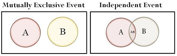
• Independent Events: Two events A and B are independent if:
  $$P(A \cap B) = P(A) \times P(B)$$
  Example: Winning a lottery and your neighbor winning a separate lottery.
• Mutually Exclusive Events: Two events that cannot happen at the same time:
  $$P(A \cap B) = 0$$
  Example: Getting a head and tail in a single toss of a coin. Example: Your 'rickshaw' and your 'metro' can't be at the same place at the same time, right?

4. Marginal, Conditional, and Joint Probability

Marginal Probability

• Marginal Probability: The probability of a single event: $P(A)$ (found by summing over the joint probabilities)

Conditional Probability

• Conditional Probability: The probability of A given B: (if $P(B) > 0$ )
  $$P(A|B) = \frac{P(A \cap B)}{P(B)}$$
  Example: Probability of getting a good score given you studied hard.

Joint Probability

• Joint Probability: The probability that both A and B occur: $P(A \cap B)$ Example: Probability of eating "samosa" and drinking "chai." Example: Like enjoying 'pakoras' more when it rains, joint events are better together!

5. Baye’s Theorem

Bayes’ Theorem

• $$P(A|B) = \frac{P(B|A) \, P(A)}{P(B)}$$
• Concept: It allows you to update the probability of an event A based on new information B.
• It's particularly useful for "predicting the cause of an event which has already occurred" or, more accurately, for revising our beliefs about the cause of an event based on new information.
• During the early stages of the COVID-19 pandemic, scientists used Bayes' Theorem to estimate the likelihood of different transmission routes (water, air, human contact) based on emerging epidemiological data. For instance, if a cluster of infections occurred in a crowded indoor space with poor ventilation, this evidence would increase the estimated probability of airborne transmission. Conversely, if no significant spread occurred in areas with treated water sources, the probability of waterborne transmission would remain low, or decrease. The theorem helped to update the probability of each transmission route, as new evidence was gathered.
• Example: Updating the chances of rain based on dark clouds.

6. Sample Vs Population

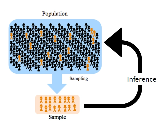
Population

• Definition: Entire group of interest.
• Mean: μ (mu)
• Variance: σ² (sigma squared)
• Example: All students in a university.

Sample

• Definition: Subset of the population.
• Mean: X̄ (x-bar)
• Variance: s² (s squared)
• Example: 100 students from the university.

Key Difference

• Population: Complete set.
• Sample: Representative subset.

Purpose

• Use sample statistics (X̄, s²) to estimate population parameters (μ, σ²).

7. Types of Data (Scales of Measurement)

1. Nominal Data:

• Definition: Categories with no inherent order.
• Example: Colors (red, blue, green), types of fruit (apple, banana, orange).

2. Ordinal Data:

• Definition: Categories with a meaningful order, but the differences between categories are not uniform.
• Example: Rating scales (poor, fair, good), education levels (high school, college, graduate).

3. Interval Data:

• Definition: Ordered data with uniform intervals, but no true zero point.
• Example: Temperature in Celsius or Fahrenheit, years.

4. Ratio Data:

• Definition: Ordered data with uniform intervals and a true zero point, allowing for meaningful ratios.
• Example: Height, weight, income, age.

8. Expectation and Variance

Expectation

• Expected Value (Discrete):
  $$E[X] = \sum x_i P(x_i)$$
  Example: The average score in a cricket match based on possible outcomes.
• Expected Value (Continuous):
  $$E[X] = \int x f(x) dx$$
• Conditional Expectation: What's the average value of X when we know that Y has a particular value y? The expected value of X given that Y equals a specific value.
  $$E[X|Y=y]$$
  Cricket Example (Runs per Over):Let X be the number of runs scored in an over. Let Y be the number of wickets that have fallen in the innings up to that over. $E[X|Y=2]$ would be the expected number of runs in an over, given that 2 wickets have fallen. $E[X|Y=8]$ would be the expected number of runs in an over, given that 8 wickets have fallen. Clearly, these two values will be different, because the number of wickets fallen influences the way the batsmen play.

Variance

• Variance: Quantifies how spread out a set of data points are around their mean (average). A high variance means the data points are widely scattered, while a low variance means they are clustered closely around the mean.
  $$Var(X) = E[X^2] - (E[X])^2$$
• Conditional Variance: Variance of a random variable X, given that another random variable Y has a specific value y. It tells you how much X varies when you know the specific value of Y.
  $$Var(X|Y=y) = E[X^2|Y=y] - (E[X|Y=y])^2$$
  Golgappa ExampleX: The number of golgappas someone can eat. Y: Their spice tolerance. Var(X): The overall variance in the number of golgappas people can eat. This will be quite high, because people have different appetites. Var(X|Y=high): The variance in the number of golgappas people can eat, given that they have high spice tolerance. This variance will be lower, because people with high spice tolerance tend to eat more golgappas, and the variations in their consumption will be less extreme. Var(X|Y=low): The variance in the number of golgappas people can eat, given that they have low spice tolerance. This variance will also be lower, but the average number of golgappas eaten will be lower than the high spice tolerance group.

9. Measures of Central Tendency & Dispersion

Central Tendency

• Mean (Average):
  $$\mu = \frac{\sum_{i=1}^{n} x_i}{n}$$
• Median: The middle value in a sorted list.
  • Odd Number of Data Points:
    $$\text{Value at } \frac{n+1}{2} \text{th position}$$
  • Even Number of Data Points:
    $$\frac{\text{Value at } \frac{n}{2} \text{th position} + \text{Value at } (\frac{n}{2} + 1) \text{th position}}{2}$$
• Mode: The most frequent value.

Dispersion

• Variance:
  $$\sigma^2 = \frac{\sum_{i=1}^{n} (x_i - \mu)^2}{n}$$
• Standard Deviation:
  $$\sigma = \sqrt{\sigma^2}$$
  Example: If data points were 'chai' cups, the mean is your average 'chai' consumption, while the standard deviation shows who's had a 'masala chai' overdose!

10. Correlation and Covariance

Covariance:

• Measures how two variables vary together.
• Covariance tells you how two variables change together.
• It's like asking: "When X goes up, does Y tend to go up too? Or does it tend to go down?"
  $$Cov(X,Y) = E[(X - \mu_X)(Y - \mu_Y)]$$
• Covariance is hard to interpret directly because its value depends on the units of the variables. A covariance of 10 could be "big" in one context and "small" in another.

Correlation:

• Correlation takes the covariance and "scales" it, so it's always between -1 and 1.
• This makes it much easier to understand the strength and direction of the relationship between two variables.
  $$\rho_{XY} = \frac{Cov(X,Y)}{\sigma_X \, \sigma_Y}$$
• A correlation of:+1 means a perfect positive relationship (X and Y go up together perfectly).
• 1 means a perfect negative relationship (X goes up, Y goes down perfectly).
• 0 means no linear relationship.
• Example: Like tracking 'chai' consumption and exam scores, more 'chai' usually means more focus (up to a point)!If we tracked how many cups of "chai" students drink (X) and their exam scores (Y), the covariance might be positive. This would mean that, in general, students who drink more "chai" tend to score higher.
• The correlation would give us a number between -1 and 1. If it's, say, 0.6, it means there's a moderately strong positive relationship.
• This is important! Correlation doesn't mean "infinite" increase. Too much "chai" might lead to jitters and actually hurt exam scores. So, the relationship might be strong up to a certain point, then weaken or reverse.

11. Random Variables

• A random variable (RV) is a numerical outcome of a random experiment.

Types:

• Discrete Random Variable: Takes countable values (e.g., number of mobile SIMs a person has).
• Continuous Random Variable: Takes an infinite number of values (e.g., height of students in an School).
• Example: "The number of times an auto driver refuses a ride in a day, discrete. The amount of time you wait for the next metro - continuous!"

12. Discrete Random Variables and Probability Mass Functions (PMFs)

• A discrete random variable (DRV) takes specific values, and its probability is given by a Probability Mass Function (PMF).

Properties of PMF

• For a DRV $X$ :

  • $P(X=x) \geq 0$ for all x.
  • $\sum P(X=x) = 1$ .

• Example: Tossing a Coin

  • Let X be the number of heads in a single toss:

    • $P(X=0) = 0.5$
    • $P(X=1) = 0.5$

• Example: "The number of golgappas a person eats before getting full. It can be 5, 10, 15, but not 7.3!"

13. Important Discrete Distributions

(a) Uniform Distribution

• A discrete uniform distribution occurs when all outcomes are equally likely.

• PMF:

  $$P(X=x) = \frac{1}{n}$$
  for $x \in {x_1, x_2, ..., x_n}$ .

• Example: A fair die roll (each number from 1 to 6 has probability 1/6).

• Example: "Choosing a random samosa from a tray where all look equally delicious, each samosa has the same chance of being picked!"

(b) Bernoulli Distribution

• A Bernoulli random variable has two possible outcomes (success = 1, failure = 0).

• PMF:

  $$P(X=x) = p^x (1-p)^{1-x}, \quad x \in {0,1}$$
  .

• Mean: $p$ .

• Variance: $p(1 - p)$ .

• Example: "Whether a student cracks UPSC in the first attempt (1 = success, 0 = failure)."

(c) Binomial Distribution

• A binomial random variable is the number of successes in n independent Bernoulli trials.

• PMF:

  $$P(X=k) = \binom{n}{k} p^k (1-p)^{n-k}$$
  .

• Mean: $np$ .

• Variance: $np(1 - p)$ .

• Example: "Number of people in a family of 5 who vote in elections, assuming each person independently decides with probability 0.7."

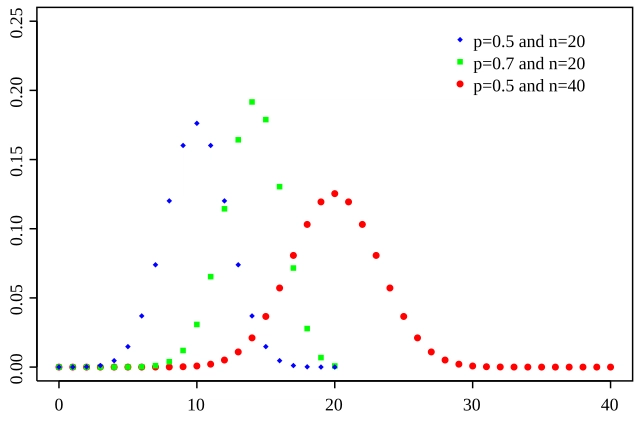
(Binomial PMF for different values of p)

14. Continuous Random Variables and Probability Density Function (PDFs)

• A continuous random variable (CRV) takes an infinite number of values. Instead of a PMF, we define a Probability Density Function (PDF).

Properties of PDFs:

• $$P(a \leq X \leq b) = \int_{a}^{b} f(x) dx$$
  (area under the curve).
• Total Probability:
  $$\int_{-\infty}^{\infty} f(x) dx = 1$$
  .
• Example: "The waiting time for an Ola ride near you is a continuous variable - you can wait 2.4 mins, 5.7 mins, etc."

15. Important Continuous Distributions

(a) Uniform Distribution (Continuous Case)

• PDF:
  $$f(x) = \frac{1}{b - a}, \quad a \leq x \leq b$$
  .
• Mean:
  $$\frac{a + b}{2}$$
  .
• Variance:
  $$\frac{(b - a)^2}{12}$$
  .
• Example: "The quality of 'pani puri' from a street vendor is uniformly distributed. Every 'puri' is equally likely to be either a masterpiece of flavor or a soggy, spicy disaster. You're taking a gamble with every bite!"

(b) Poisson Distribution

• The Poisson distribution models the number of events occurring in a fixed time or space.

• PMF:

  $$P(X=k) = \frac{\lambda^k e^{-\lambda}}{k!}, k = 0, 1, 2, ...$$

• Mean & Variance: $λ$

• Example: "The number of people entering a Mumbai local train in one minute follows a Poisson distribution, sometimes few, sometimes an entire village at once!"

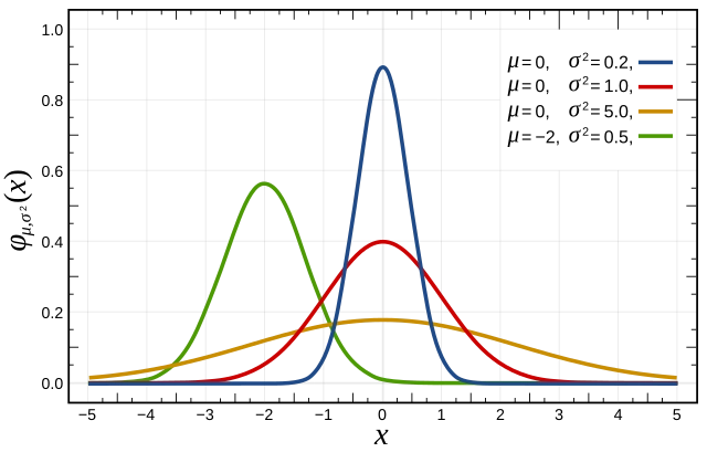
(c) Normal (Gaussian) Distribution

• The normal distribution is the most important probability distribution.

• PDF:

  $$f(x) = \frac{1}{\sqrt{2\pi \sigma^2}} e^{-\frac{(x - \mu)^2}{2\sigma^2}}$$
  .

• Mean: $\mu$ .

• Variance: $\sigma^2$ .

• Example: "The number of 'chai' breaks a typical Indian office employee takes in a day follows a normal distribution. Most employees hover around the average number of breaks (usually quite high), with a few 'chai' enthusiasts at the extreme high end and a rare breed of 'chai'-avoiders at the low end. The boss, of course, believes it should be a very narrow normal distribution centered around 'zero breaks,' but reality has other plans!"

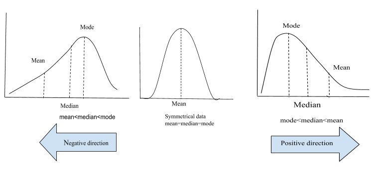
Skewness

• Definition: Skewness measures the asymmetry of a probability distribution. In a perfectly symmetrical normal distribution, skewness is zero.
• Types:
  • Positive Skew (Right Skew): The tail on the right side is longer, and the mass of the distribution is concentrated on the left. Mean > Median > Mode.
  • Negative Skew (Left Skew): The tail on the left side is longer, and the mass of the distribution is concentrated on the right. Mean < Median < Mode.
  • Zero Skew: The distribution is symmetrical.
• Formula (Sample Skewness):
  $$g_1 = \frac{\frac{1}{n} \sum_{i=1}^{n} (x_i - \bar{x})^3}{s^3}$$

• Normal Distribution Skewness: For a perfectly normal distribution, skewness is 0.

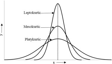
Kurtosis

• Definition: Kurtosis measures the "tailedness" of a probability distribution. It describes the shape of the tails of the distribution.
• Types:
  • Leptokurtic (Positive Excess Kurtosis): Distributions with heavy tails and a sharp peak. Kurtosis > 3.
  • Mesokurtic (Normal Kurtosis): Distributions with moderate tails. Kurtosis = 3. The normal distribution is mesokurtic.
  • Platykurtic (Negative Excess Kurtosis): Distributions with thin tails and a flat peak. Kurtosis < 3.
• Formula (Sample Kurtosis):
  $$g_2 = \frac{\frac{1}{n} \sum_{i=1}^{n} (x_i - \bar{x})^4}{s^4} - 3$$
• Excess Kurtosis: The "-3" in the formula is to make the kurtosis of the normal distribution equal to 0. Therefore, the result of the formula is called excess kurtosis.

• Normal Distribution Kurtosis: For a normal distribution, the kurtosis is 3. However, the excess kurtosis is 0.

(d) Standard Normal Distribution

• The standard normal distribution is a normal distribution with mean = 0 and variance = 1.

• Z-score:

  $$Z = \frac{X - \mu}{\sigma}$$

• Example: "Imagine converting every student's JEE percentile to a common scale, this is what the Z-score does in statistics!"

(e) Exponential Distribution

• Models the time between independent events happening at a constant rate.

• PDF:

  $$f(x) = \lambda e^{-\lambda x}, \quad x \geq 0$$
  .

• Mean:

  $$\frac{1}{\lambda}$$
  .

• Variance:

  $$\frac{1}{\lambda^2}$$
  .

• Example: "The time between your neighbor's unexpected 'guests' dropping by for 'chai' and 'gup-shup' follows an exponential distribution. You know they'll come eventually, but you never know exactly when. It's like waiting for a rickshaw in a busy market, you just hope it's soon, and that it's going your way!"

(f) Student's t-Distribution

• Used when sample sizes are small and population variance is unknown. It has fatter tails than a normal distribution.

• PDF:

  $$f(x) = \frac{\Gamma(\frac{\nu+1}{2})}{\sqrt{\nu\pi} \Gamma(\frac{\nu}{2})} \left( 1 + \frac{x^2}{\nu} \right)^{-\frac{\nu+1}{2}}$$

• Mean: 0, Variance:

  $$\frac{\nu}{\nu - 2}$$
  for $\nu > 2$ .

• Example: "When calculating the average marks of a small sample of IIT aspirants, we use t-distribution because we don't know the true population variance!"

(g) Chi-Squared (χ²) Distribution

• The sum of the squares of k independent standard normal variables follows a Chi-squared distribution.

• PDF:

  $$f(x) = \frac{x^{(k/2) - 1} e^{-x/2}}{2^{k/2} \Gamma(k/2)}, x > 0$$

• Mean: $k$ , Variance: $2k$ .

• Example: "Chi-squared tests are often used to check if cricket team selection is truly random or biased!"

(h) Cumulative Distribution Function (CDF)

• The Cumulative Distribution Function (CDF) gives the probability that a random variable X is less than or equal to a value x.

• Formula:

  $$F(x) = P(X \leq x) = \int_{-\infty}^{x} f(t) dt$$

• For Discrete:

  $$F(x) = \sum_{t \leq x} P(X = t)$$

• Example: "If the probability of reaching college on time depends on the time you leave, the CDF shows how early you should leave to have a 90% chance of being on time!"

16. Conditional Probability Density Function (Conditional PDF)

• The conditional PDF describes the probability distribution of X given that another variable Y has taken a certain value.

• Formula (Continuous Case):

  $$f_{X|Y}(x | y) = \frac{f_{X,Y}(x,y)}{f_Y(y)}$$

• where $f_{X,Y}(x,y)$ is the joint PDF, and $f_Y(y)$ is the marginal PDF.

• Example: "The probability of getting an auto in Bengaluru depends on whether it is raining. If it rains, the probability drops to near zero, unless you are willing to pay double!"

I'll convert all the inline mathematical equations in this content to use the {% katex inline %} format. Here's the converted text:

17. Central Limit Theorem (CLT)

• The Central Limit Theorem states that the sum (or average) of a large number of independent random variables tends to follow a normal distribution, regardless of the original distribution.

• Mathematically: If $X_1,X_2,......X_n$ are i.i.d. (independent and identically distributed) random variables with mean μ and variance σ², then as n → ∞:
  

  $$\frac{\sum_{i=1}^{n} X_i - n\mu}{\sqrt{n\sigma^2}} \approx \mathcal{N}(0,1)$$

• Example: "If 100 people from different cities taste Hyderabadi biryani, their average rating will be normally distributed, even if individual ratings range from 'best biryani ever' to 'no spice, no life!'"

18. Confidence Interval (CI)

• A confidence interval gives a range within which we expect a population parameter (like the mean) to lie, with a certain level of confidence (e.g., 95%).

• Formula for Mean (Known Variance):
  

  $$\bar{X} \pm Z_{\alpha/2} \times \frac{\sigma}{\sqrt{n}}$$
  where $Z_{\alpha/2}$ is the critical value for confidence level (1-α), σ is the standard deviation, and n is the sample size.

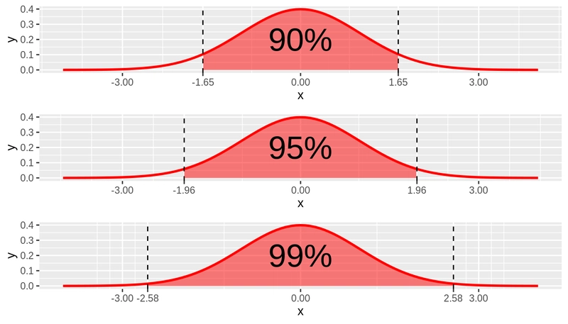
• Example: "A stadium manager estimates that 30,000 to 35,000 people will attend the India-Pakistan cricket match, with a 90% confidence interval. This means there's a 10% chance that either nobody shows up because of a sudden flood, or that the entire population of the city tries to squeeze in!"

19. Important Tests

Parametric vs. Non-Parametric Tests

Parametric Tests:

• Assumptions: These tests assume that the data follows a specific distribution, typically a normal distribution. They also often assume homogeneity of variances.
• Data Type: Generally used with interval or ratio data.
• Advantages: More powerful when assumptions are met.
• Examples: Z-test, t-test, ANOVA, Pearson's correlation, linear regression.

Non-Parametric Tests:

• Assumptions: These tests make fewer assumptions about the underlying distribution of the data. They are often used when data is not normally distributed or when dealing with ordinal or nominal data.
• Data Type: Can be used with ordinal, nominal, or non-normally distributed interval/ratio data.
• Advantages: Robust to violations of assumptions, suitable for smaller sample sizes.
• Examples: Chi-squared test, Mann-Whitney U test, Wilcoxon signed-rank test, Kruskal-Wallis test.

Parametric Tests

Z-Test

• Purpose: Compare sample mean to population mean when population variance is known and sample size is large (n > 30).
• Formula:
  $$Z = \frac{\bar{X} - \mu}{\sigma / \sqrt{n}}$$
• Example: "A scientist checks if Mumbai's average air particulate matter exceeds a known historical standard, using a large dataset."

T-Test

• Purpose: Compare sample means when population variance is unknown, especially with small samples (n < 30).
• Formula (One-Sample t-test):
  $$t = \frac{\bar{X} - \mu}{s / \sqrt{n}}$$
• Types:
  • One-Sample: Sample mean vs. known population mean.
  • Two-Sample (Independent): Compare means of two independent groups.
  • Paired: Compare means of the same group before and after a treatment.
• Example: "Comparing average weight of hostel students before and after Diwali (paired t-test)."

ANOVA (Analysis of Variance)

• Purpose: Compare means of three or more groups.
• Formula (One-Way ANOVA, F-statistic):
  $$F = \frac{MS_{between}}{MS_{within}}$$
• Example: "Testing if different fertilizer types significantly affect rice yield in Punjab."

Correlation Test (Pearson's r)

• Purpose: Measure the linear relationship between two continuous variables.
• Formula:
  $$r = \frac{\sum (x_i - \bar{x})(y_i - \bar{y})}{\sqrt{\sum (x_i - \bar{x})^2 \sum (y_i - \bar{y})^2}}$$
• Example: "Checking if study hours correlate with exam scores in a university."

Regression Analysis (Linear)

• Purpose: Model the linear relationship between dependent and independent variables.
• Formula (Simple Linear Regression):
  $$y = a + bx$$
• Example: "Predicting apartment prices in Mumbai based on size and location."

Shapiro-Wilk Test

• Purpose: Test for normality of data distribution.
• Example: "Checking if daily rainfall in Chennai follows a normal distribution."

Non-Parametric Tests

Chi-Squared (χ²) Test

• Purpose: Test independence between categorical variables or goodness of fit.
• Formula:
  $$\chi^2 = \sum \frac{(O - E)^2}{E}$$
• Types:
  • Goodness of Fit: Compare observed vs. expected frequencies.
  • Test for Independence: Determine if two categorical variables are related.
• Example: "Testing if favorite cricket team is related to home state (e.g., CSK fans from Tamil Nadu)."

Mann-Whitney U Test

• Purpose: Compare two independent groups (ordinal or non-normally distributed continuous data).
• Example: "Comparing median income of rural vs. urban households."

Wilcoxon Signed-Rank Test

• Purpose: Compare paired data (ordinal or non-normally distributed continuous data).
• Example: "Comparing stress levels before and after a yoga program."

Kruskal-Wallis Test

• Purpose: Compare three or more independent groups (ordinal or non-normally distributed continuous data).
• Example: "Testing if spice levels differ across North, South, and East Indian cuisines."

20. Hypothesis Testing: A Deeper Dive

1. Null Hypothesis (H₀)

• Definition: The statement of "nothing's changed" or "no difference exists." It's what we assume to be true until proven otherwise.
• Example: "H₀: The average 'aloo paratha' in Punjab has the same amount of 'aloo' filling as anywhere else." (The assumption that regional differences don't exist.)

2. Alternative Hypothesis (H₁)

• Definition: The statement that contradicts the null hypothesis. It's what we're trying to prove.
• Example: "H₁: Punjabi 'aloo parathas' have significantly more 'aloo' filling." (The hungry traveler's hope.)

3. P-value

• Definition: The probability of getting the observed results (or more extreme) if the null hypothesis were true. A small P-value means we have strong doubt about the null hypothesis.
• Example: "If the P-value is 0.0001 when testing 'aloo' filling, it means there is a 0.01% chance that all parathas have the same amount of filling. "

4. Significance Level (α)

• Definition: A pre-determined threshold (usually 0.05) used to decide whether to reject the null hypothesis. If the P-value is less than α, we reject H₀.
• Example: "If we set α = 0.01, it means we want to be 99% sure that the parathas are different"

5. Type I Error

• Definition: Concluding there's a difference when there isn't.
• Example: "A tourist claims that the parathas are different when they aren't, because they are just too hungry."

6. Type II Error

• Definition: Concluding there's no difference when there is.
• Example: "A food critic fails to notice that the parathas are different, and doesn't tell the world about the best paratha in the world."

Gistr | Highlight and share the best insights from YouTube videos

Stop watching YouTube videos mindlessly. Transform them into AI-powered notes and highlights that you can curate and share. Perfect for students, professionals, and researchers.

gistr.so