
Algorithm Complexity and Big O Notation
Objective: In this lesson, we'll cover the topics of Algorithm Complexity and Big O Notation. By the end, you should:
- Be familiar with these terms and what they mean.
- See their use in practice.
- Use these tools to measure how "good" an algorithm is.
This lesson was originally published at https://algodaily.com, where I maintain a technical interview course and write think-pieces for ambitious developers.
In software engineering, developers can write a program in several ways.
For instance, there are many ways to search an item within a data structure. You can use linear search, binary search, jump search, interpolation search, among many other options.
Our focus in this lesson is on mastering Algorithm Complexity and Big O Notation. But what we want to do with this knowledge is to improve the performance of a software application. This is why it's important to understand which algorithm to use, depending upon the problem at hand.
Let's start with basics. A computer algorithm is a series of steps the machine takes in order to compute an output. There are several ways to measure its performance. One of the metrics used to compare algorithms is this notion of algorithm complexity.
Sounds challenging, doesn't it? Don't worry, we'll break it down.
Algorithm complexity can be further divided into two types: time complexity and space complexity. Let's briefly touch on these two:
- The time complexity, as the name suggests, refers to the time taken by the algorithm to complete its execution.
- The space complexity refers to the memory occupied by the algorithm.
In this lesson, we will study time and space complexity with the help of many examples. Before we jump in, let’s see an example of why it is important to measure algorithm complexity.
Importance of Algorithm Complexity
To study the importance of algorithm complexity, let’s write two simple programs. Both the programs raise a number x to the power y.
Here's the first program: see the sample code for Program 1.
def custom_power(x, y):
    result = 1
    for i in range(y):
        result = result * x
    return result

print(custom_power(3, 4))
Let’s now see how much time the previous function takes to execute. In Jupyter Notebook or any Python interpreter, you can use the following script to find the time taken by the algorithm.
from timeit import timeit

func = '''
def custom_power(x, y):
    result = 1
    for i in range(y):
        result = result * x
    return result
'''

t = timeit("custom_power(3,4)", setup=func)
print(t)
You'll get the time of execution for the program.
I got the following results from running the code.
600 ns ± 230 ns per loop (mean ± std. dev. of 7 runs, 1000000 loops each)
Let's say that the custom_power function took around 600 nanoseconds to execute. We can now compare with program 2.
Program 2:
Let’s now use the Python’s built-in pow function to raise 3 to the power 4 and see how much time it ultimately takes.
from timeit import timeit

t = timeit("pow(3, 4)")
print(t)
Again, you'll see the time taken to execute. The results are as follows.
308 ns ± 5.03 ns per loop (mean ± std. dev. of 7 runs, 1000000 loops each)
Please note that the built-in function took around 308 nanoseconds.
What does this mean?
You can clearly see that Program 2 is twice as fast as Program 1. This is just a simple example. However if you are building a real-world application, the wrong choice of algorithms can result in sluggish and inefficient user experiences. Thus, it is very important to determine algorithm complexity and optimize for it.
Big(O) Notation
Let's now talk about Big(O) Notation. Given what we've seen, you may ask-- why do we need Big O if we can just measure execution speed?
In the last section, we recorded the clock time that our computer took to execute a function. We then used this clock time to compare the two programs. But clock time is hardware dependent. An efficient program may take more time to execute on a slower computer than an inefficient program on a fast computer.
So clock time is not a good metric to find time complexity. Then how do we compare the algorithm complexity of two programs in a standardized manner? The answer is Big(O) notation.
Big(O) notation is an algorithm complexity metric. It defines the relationship between the number of inputs and the step taken by the algorithm to process those inputs. Read the last sentence very carefully-- it takes a while to understand. Big(O) is NOT about measuring speed, it is about measuring the amount of work a program has to do as an input scales.
We can use Big(O) to define both time and space complexity. The below are some of the examples of Big(O) notation, starting from "fastest"/"best" to "slowest"/"worst".
| Function | Big(O) Notation |
| Constant | O(c) |
| Logarithmic | O(log(n)) |
| Linear | O(n) |
| Quadratic | O(n^2) |
| Cubic | O(n^3) |
| Exponential | O(2^n) |
Let’s see how to calculate time complexity for some of the aforementioned functions using Big(O) notation.
Big(O) Notation for Time Complexity
In this section we will see examples of finding the Big(O) notation for certain constant, linear and quadratic functions.
Constant Complexity
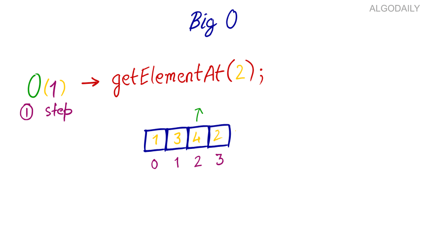
In the constant complexity, the steps taken to complete the execution of a program remains the same irrespective of the input size. Look at the following example:
import numpy as np

def display_first_cube(items):
    result = pow(items[0],3)
    print (result)

inputs = np.array([2,3,4,5,6,7])
display_first_cube(inputs)
In the above example, the display_first_cube element calculates the cube of a number. That number happens to be the first item of the list that passed to it as a parameter. No matter how many elements there are in the list, the display_first_cube function always performs two steps. First, calculate the cube of the first element. Second, print the result on the console. Hence the algorithm complexity remains constant (it does not scale with input).
Let’s plot the constant algorithm complexity.
import numpy as np
import matplotlib.pyplot as plt

num_of_inputs = np.array([1,2,3,4,5,6,7])
steps = [2 for n in num_of_inputs]

plt.plot(num_of_inputs, steps, 'r')
plt.xlabel('Number of inputs')
plt.ylabel('Number of steps')
plt.title('O(c) Complexity')

plt.show()
In the above code we have a list num_of_inputs that contains a different number of inputs. The steps list will always contain 2 for each item in the num_of_inputs list. If you plot the num_of_inputs list on x-axis and the steps list on y-axis you will see a straight line as shown in the output:

Linear Complexity*
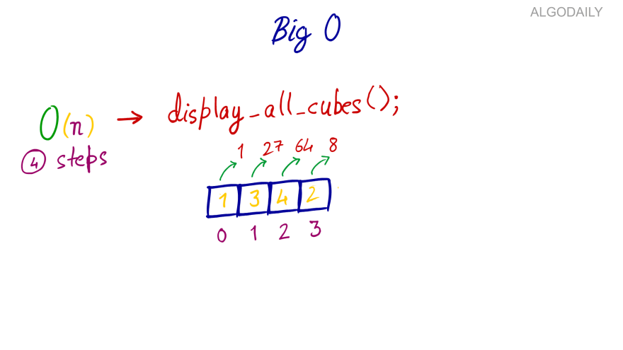
In functions or algorithms with linear complexity, a single unit increase in the input causes a unit increase in the steps required to complete the program execution.
A function that calculates the cubes of all elements in a list has a linear complexity. This is because as the input (the list) grows, it will need to do one unit more work per item. Look at the following script.
import numpy as np

def display_all_cubes(items):
    for item in items:
        result = pow(item,3)
        print (result)

inputs = np.array([2,3,4,5,6,7])
display_all_cubes(inputs)
For each item in the items list passed as a parameter to display_all_cubes function, the function finds the cube of the item and then displays it on the screen. If you double the elements in the input list, the steps needed to execute the display_all_cubes function will also be doubled. For the functions, with linear complexity, you should see a straight line increasing in positive direction as shown below:

num_of_inputs = np.array([1,2,3,4,5,6,7])
steps = [2*n for n in no_inputs]

plt.plot(no_inputs, steps, 'r')
plt.xlabel('Number of inputs')
plt.ylabel('Number of steps')
plt.title('O(n) Complexity')
plt.show()
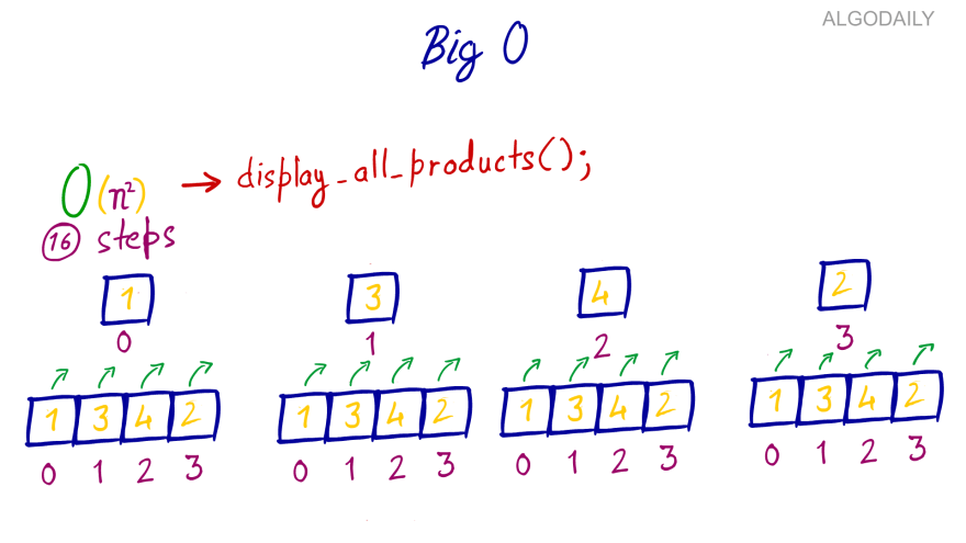
Quadratic Complexity
As you might guess by now-- in a function with quadratic complexity, the output steps increase quadratically with the increase in the inputs. Have a look at the following example:
import numpy as np

def display_all_products(items):
    for item in items:
        for inner_item in items:
            print(item * inner_item)

inputs = np.array([2,3,4,5,6])
display_all_products(inputs)
In the above code, the display_all_products function multiplies each item in the “items” list with all the other elements.
The outer loop iterates through each item, and then for each item in the outer loop, the inner loop iterates over each item. This makes total number of steps n x n where n is the number of items in the “items” list.
If you plot the inputs and the output steps, you should see the graph for a quadratic equation as shown below. Here is the output:
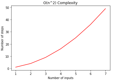
num_of_inputs = np.array([1,2,3,4,5,6,7])
steps = [pow(n,2) for n in no_inputs]

plt.plot(no_inputs, steps, 'r')
plt.xlabel('Number of inputs')
plt.ylabel('Number of steps')
plt.title('O(n^2) Complexity')
plt.show()
Here no matter the size of the input, the display_first_cube has to allocate memory only once for the result variable. Hence the Big(O) notation for the space complexity of the “display_first_cube” will be O(1) which is basically O(c) i.e. constant.
Similarly, the space complexity of the display_all_cubes function will be O(n) since for each item in the input, space has to be allocated in memory.
Big(O) Notation for Space Complexity
To find space complexity, we simply calculate the space (working storage, or memory) that the algorithm will need to allocate against the items in the inputs. Let’s again take a look at the display_first_cube function.
import numpy as np

def display_first_cube(items):
    result = pow(items[0],3)
    print (result)

inputs = np.array([2,3,4,5,6,7])
display_first_cube(inputs)
Best vs Worst Case Complexity
You may hear the term worst case when discussing complexities.
An algorithm can have two types of complexities. They are best case scenarios and worst case scenarios.
The best case complexity refers to the complexity of an algorithm in the ideal situation. For instance, if you want to search an item X in the list of N items. The best case scenario is that we find the item at the first index in which case the algorithm complexity will be O(1).
The worst case is that we find the item at the nth (or last) index, in which case the algorithm complexity will be O(N) where n is the total number of items in the list. When we use the term algorithmic complexity, we generally refer to worst case complexity. This is to ensure that we are optimizing for the least ideal situation.
Conclusion
Algorithm complexity is used to measure the performance of an algorithm in terms of time taken and the space consumed.
Big(O) notation is one of the most commonly used metrics for measuring algorithm complexity. In this article you saw how to find different types of time and space complexities of algorithms using Big(O) notation. You'll now be better equipped to make trade-off decisions based on complexity in the future.
This lesson was originally published at https://algodaily.com, where I maintain a technical interview course and write think-pieces for ambitious developers.

Top comments (0)