

The Defective Chessboard problem, also known as the Tiling Problem is an interesting problem. It is typically solved with a “divide and conquer” approach. The algorithm has a time complexity of O(n²).
The problem
Given a n by n board where n is of form 2^k where k >= 1 (Basically, n is a power of 2 with minimum value as 2). The board has one missing square). Fill the board using trionimos. A trionimo is an L-shaped tile is a 2 × 2 block with one cell of size 1×1 missing.
Solving the problem efficiently isn’t the goal of this post. Visualizing the board as the algorithm runs is much more interesting in my opinion, though. Lets discuss the algorithm first.
The Algorithm
As mentioned earlier, a divide-and-conquer (DAC) technique is used to solve the problem. DAC entails splitting a larger problem into sub-problems, ensuring that each sub-problem is an exact copy of the larger one, albeit smaller. You may see where we are going with this, but lets do it explicitly.
The question we must ask before writing the algorithm is: is this even possible? Well, yes. The total number of squares on our board is n², or 4^k. Removing the defect, we would have 4^k — 1, which is always a multiple of three. This can be proved with mathematical induction pretty easily, so I won’t be discussing it.
The base case
Every recursive algorithm must have a base case, to ensure that it terminates. For us, lets consider the case when n, 2^k is 2. We thus have a 2×2 block with a single defect. Solving this is trivial: the remaining 3 squares naturally form a trionimo.
The recursive step
To make every sub-problem a smaller version of our original problem, all we have to do is add our own defects, but in a very specific way. If you take a closer look, adding a “defect” trionimo at the center, with one square in each of the four quadrants of our board, except for the one with our original defect would allow use to make four proper sub-problems, at the same time ensuring that we can solve the complete problem by adding a last trionimo to cover up the three pseudo-defective squares we added.
Once we are done adding the “defects”, recursively solving each of the four sub-problems takes us to our last step, which was already discussed in the previous paragraph.
The combine step
After solving each of the four sub-problems and putting them together to form a complete board, we have 4 defects in our board: the original one will lie in one of the quadrants, while the other three were those we had intentionally added to solved the problem using DAC. All we have to do is add a final trionimo to cover up those three ‘defects’ and we are done.
Thus, the recursive equation for time complexity becomes:
T(n) = 4T(n/2)+c
The 4 comes from the fact that to solve each problem of input n, we divide it into 4 sub-problems of input size n/2 (half the length of the original board). Once we are done solving those sub-problems, all that’s left to be done is to combine them: this is done by adding the last trionimo to cover up the pseudo-defects we added. This, of course, is done in constant time.
If you are interested in finding the asymptotic time complexity of the recurrence relation, you could try the recursion tree method or the substitution method. For now, lets just use the Master theorem.
The master theorem says that for a recurrence relation of the form:
T(n) = aT(n/b) + f(n)
the complexity depends on the complexities of f(n) and n ^ log_b(a) (the log is to the base b).
The cases in the image below tell us which case we need to use here.
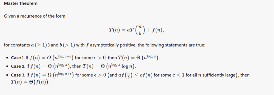
Since the value of n ^ log(a) base b is n², while the term f(n) is of constant complexity, we use Case 1, which ultimately tells us that our algorithm has an order of n². In other words, the time complexity of our algorithm is O(n²).
The Code
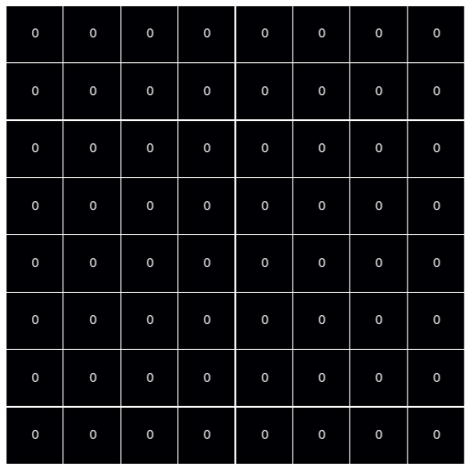
Initially, each square is represented by a 0. A ‘-1’ represents a defective square, and would appear black in the plots. Each trionimo would be displayed with a unique number, which would be incremented as more trionimos are added.
Again, the goal of the code is not optimization — its to do as much from scratch (in plain python) as possible.
I have commented the code below, so it should be pretty straight-forward.
Importing required libraries
The random library is used to randomly pick a square to be defective, just for starting the problem, and seaborn is, of course, for the visualization.
Creating the board
Nothing too crazy: just creating a two dimensional Python list. The algorithm can be optimized by using structures like numpy arrays instead of vanilla Python lists. The list is initialized with 0's.
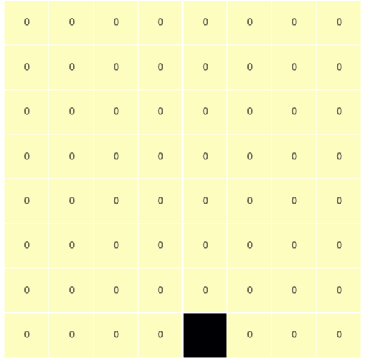
Adding a defect randomly
Here we are randomly choosing an element using randint() and making it the defective tile. We will represent defects with a -1.
Locating the defect when solving each sub-problem
We are doing two things here:
- locating the row and column of the defect
- determining which quadrant of the board the defect lies in
The first step can be optimized by using numpy functions instead of the ‘from-scratch’ approach below.
Adding trionimos
This function adds a trionimo to a 2 x 2 section of the board. Here, the quadrant of the defect comes in handy as we can simply define a dictionary to decide how to add our trionimo.
Recursive Tiling Function
This is a divide-and-conquer implementation of our tiling algorithm. The function accomplishes the following:
- determining the location of the defect in the given section of the board (the rows r1 and r2 and the columns c1 and c2 allow the function to focus on a particular section of the board).
- adding a trionimo if we are dealing with a 2 x 2 section of the board
- otherwise, adding three defects to the center
- recursively solving each quadrant of the board
- adding a final trionimo to cover up the three defects we added at the center.
The Parent Tiling Function
This just makes the interface cleaner since we technically have only two independent arguments: the board and the parameter k (well, k can be calculated or used as a global variable, but that’s up to the programmer).
Visualizing
I made use of a simple seaborn heat-map to display the board. The drawboard() method creates the heat-map.
The two heat-map calls are to more easily distinguish between defective and non-defective squares:
- the first one creates the heat-map without any labels or masks.
- the second heat-map has a mask which hides the defective squares, but annotates the rest, allowing us to distinguish each trionimo by number while leaving defective squares blank.
The result
I’ve dragged the post long enough. The snippet below calls relevant functions, allowing us to view each of the board’s states.
Originally published at https://polaris000.github.io on January 11, 2020.

Top comments (0)