From scraping in the cloud to streams of insights

Any questions? Please comment and let me know what you think!

Before going into story-telling, this post touches on the following topics - please, jump ahead:

• Caching data
• Corner-cases on Wikipedia
• Missing elevation data on Wikidata
• Extensible storage of facts
• Dual-axis weather plots
• Running circles around airports
• Gift ribbon for Google cloud-functions
• Hiding input in automatic reports from Jupyter notebooks
• Results
• I did not do it

---

Or, just read it front-to-back:

I am currently enrolled in a WBS Coding School Data Science Boot Camp and the past two weeks, we were learning the data-engineering skills of ETL, i.e. extraction, transformation and loading of data into storage for comprehensive analysis.

As learning scenario, we thought of a fictitious E-scooter rental company called Gans which is interested in up-to-date information on the cities they operate in such that they can plan their work better. Two points were of particular interest:

• weather data in order to anticipate less busy times for maintenance
• flight data in order to accommodate for higher demand in certain parts of the city

Caching data

In this project, we were using the two most common methods of acquiring data:

• scraping information from unstructured web-pages
• requesting structured data from APIs

Both of those are relatively slow operations that can limit development turnaround when you are still working on the details of post-processing and storing the data in the framework of a Jupyter notebook. Also, APIs usually put limits on the number of requests, you can do, and web-sites might get annoyed and ban you for too frequent requests.

To address this, it is quite easy to implement caching logic. I used a custom attribute on my data-retrieval function which seems to be the closest Python-analogy to function-static variables that I know from C++. We were using Beautiful Soup for parsing the HTML and it looks like this:

import requests
from bs4 import BeautifulSoup
from datetime import datetime

scrape_list = []
use_caching = True

def get_soup(url: str):
  """
  Retrieve HTML soup from URL using a local soup cache.

  If the URL was previously retrieved, the cached soup is 
  served instead of making a web request. If the URL is 
  requested from the web, the soup is stored in the cache.

  :param url: the URL to retrieve from cache or web
  :return: tuple(soup, scrape_index) 
    where scrape_index refers to the scrape_list
  """

  if use_caching:
    try:
      if cached := get_soup.cache.get(url):
        return cached
    except:
      get_soup.cache = {}

  dt = datetime.now()
  response = requests.get(url)
  soup = BeautifulSoup(response.content, 'html.parser')
  scrape_index = len(scrape_list)
  scrape_list.append([url, dt, None])
  if use_caching:
    get_soup.cache[url] = (soup, scrape_index)
  return (soup, scrape_index)

As you can see, caching is made optional because in production, when the script is run in the cloud only once per instance of time and not multiple times inside a Jupyter notebook for development purposes, it is a waste to keep all retrieved documents in memory even if they will not be used a second time.

Also, the requested URL and current time is saved in a scrape_list such that this information can be later saved to the database along with the extracted information. The third None entry in each record there is later used to hold the database ID once the scrape is stored.

I also wrote a very similar function for retrieving and caching JSON data from APIs:

def get_json(url, headers = None):
  """
  Retrieve JSON from URL using a local cache.

  If the URL was previously retrieved, the cached JSON is 
  served instead of making a web request. If the URL is 
  requested from the web, the JSON is stored in the cache.

  :param url: the URL to retrieve from cache or web
  :param headers: the HTTP request headers to pass 
    (for authorization)
  :return: tuple (json, scrape_index) 
    where scrape_index refers to the scrape_list
  """
  if use_caching:
    try:
      if cached := get_json.cache.get(url):
        return cached
    except:
      get_json.cache = {}

  dt = datetime.now()
  response = requests.get(url, headers=headers)
  response.raise_for_status()
  if response.status_code == 204: # No Content
    json = None
  else:
    json = response.json()

  scrape_index = len(scrape_list)
  scrape_list.append([url, dt, None])
  if use_caching:
    get_json.cache[url] = (json, scrape_index)
  return (json, scrape_index)

The main difference apart from parsing JSON instead of HTML and passing HTTP request headers for authorization is handling of HTTP request result states such as failures like 404 via exceptions and the special 204 No Content reply.

Corner-cases on Wikipedia

For the exercise, we extracted geographical location information and population numbers from https://en.wikipedia.org . As to be expected from unstructured data, and even though Wikipedia has some guidelines and tries to follow common patterns across the articles for different cities, the scraping function for processing Wikipedia had to be successively extended to handle certain corner-cases as I extended the list of cities, e.g. different labels or slightly different formatting of the population numbers.

Missing elevation data on Wikidata

In contrast, https://wikidata.org follows strict rules on data-structure and Wikipedia links to the corresponding Wikidata pages. This makes it quite easy to scrape data because every type of information has unique identifiers. However, not many cities actually have peak elevation data, so my initial idea on elevation data failed which was to retrieve average and highest elevation in order to estimate hilliness which is in general relevant for E-scooter use.

Extensible storage of facts

The common approach to store information like population data would be to make it a column in the city database table. In order to allow tracking change of facts over time, one could in contrast employ a separate table which stores the time of the scrape, population and other facts in multiple columns linked to the respective city such that a time-series of such information may evolve.

However, I wanted to try an approach that allows you to later on add new types of facts without changing the database table schema. Even though, some consider it an anti-pattern, I used the entity-attribute-value model to store the population data. This allows to later on add a new type of information (e.g. GDP per capita) to the measure table and then just store the new information in a fact table.

As a counter-argument to bashing this as an anti-pattern: Each time, you do an evaluation of your facts based on a current set of measures, it is quite easy to write a common table expression that transforms your fact table into a classical table with individual columns for each of your measures just as you had designed it otherwise but without having to update the database schema each time you add a new measure. You just need to update your evaluation code.

As an example how to assemble the fact data into a classical table, see this and the SQL schema for reference:

WITH latest_fact AS (
  SELECT * FROM fact f1
  WHERE NOT EXISTS( -- a newer value for the same fact:
    SELECT 1 FROM fact f2
    WHERE f2.city = f1.city
    AND f2.measure = f1.measure
    AND f2.scrape > f1.scrape
  )
),
city_facts AS (
  SELECT name AS city, 
    -- convert string to number:
    population.value + 0 AS population,
    population.meta AS population_meta, 
    population_scrape.timestamp AS population_scrape_timestamp
  FROM city
  LEFT JOIN latest_fact population 
    ON population.measure = (
      SELECT id FROM measure WHERE name = 'population'
    )
    AND population.city = city.id
  LEFT JOIN scrape population_scrape
    ON population_scrape.id = population.scrape
)
SELECT city, 
  population, 
  population_meta->"$.date" AS census_date
FROM city_facts
ORDER BY population DESC
;

Here city_facts is a classical table-representation of the latest known facts. The population_meta is a JSON-column for case-dependent meta-data about that fact (census-date of reference in the example of population data). The city_facts can then be queried to give a result like this:

city	population	census_date
New York City	8804190	2020
London	8799800	2021
Sydney	5297089	2022
Berlin	3850809	2021
Paris	2102650	2023
Vienna	2002821
Hamburg	1945532	2022-12-31

Dual-axis weather plots

Retrieving weather data from the OpenWeather API was straight-forward. We could use the previously retrieved latitude/longitude coordinates for the cities. I focused on saving values that seemed relevant for E-scooter use like felt temperature, rain, snow, wind and wind gusts. My primary visualization for this would be per-city plots showing temperature and precipitation which requires two different y-axes in the same plot and cannot be achieved with seaborn's convenient but opinionated "figure-level" API. So, I had to dive a bit deeper to come up with figures like this:

I quite like how you can see the transition between rain and snow in some cases. Placing the legend was a bit of a challenge.

Running circles around airports

For flight-data, we were using the AeroDataBox API. There were a few peculiarities to take into account here:

• the API would only give you flight data for a maximum span of 12h, so covering a full day and night would take two requests
• the API would expect times given only in the airport's local time-zone, so aligning the data in common UTC would require time-zone conversion

Fortunately, using the timezonefinder package made it quite easy to identify the timezone from the airport coordinates reported by AeroDataBox.

Because airports tend to be far out of the city center where E-scooter business is going on, I assumed that commuting to the airport would be done by car, cab or public transport and the effect on E-scooter use would happen with a time-shift w.r.t. the arrival and departure times of flights. These time-shifts would depend on estimated quantities like how early people tend to arrive at the airport ahead of flights and how long it takes them to pick up baggage, clear immigration and walk out of the building but also the commuting time to and from the airport. To estimate this, I used an average city travel speed and the distance between airport and city center which I calculated using the GeoPy ellipsoidal distance calculation module.

Also, some cities have multiple airports in their vicinity and some airports have multiple cities in their vicinity which makes the calculations necessary for each pair and then to accumulate the results.

Again, I was too demanding for poor seaborn's convenient but opinionated "figure-level" API that I had to counter-act a bit to get back to well-formatted x-axis ticks on all and not only the bottom sub-figures because, you know, when there are lots of figures, you won't see the bottom row and some x-axis visible is quite helpful, really.

Sorry, for the tiny bit of ranting but this is what the results look like:

I like that you can easily see that E-scooter use for departures of course is expected to happen earlier than for arrivals in general and how different the distribution is for the cities of Tübingen and Stuttgart which are both served by Stuttgart airport but have different commute times. The individual shape differences are caused by the different per-hour binning.

The counts mean expected users based on an average number of passengers per flight and a global fraction of E-scooter users per flight.

Gift ribbon for Google cloud-functions

As I was happy with having all the extraction-transformation-load logic being refactored into self-containing units and a central orchestrating function, it was time to wrap this logic into a Google cloud-function container and have it run at periodic intervals.

The main challenge was to come up with a comprehensive list of utilized Python packages in requirements.txt. As helpers, I found pipreqs and the recommendation to use it along with pip-compile from pip-tools. And, yes, that's a nice start but there are dynamic things that are not picked up by these tools like the actually used SQL driver in SQLAlchemy (pymysql) or the IPython kernel itself for running Jupyter notebooks (see below).

Anyway, to deserve it, you need to work a little. So, no complaints here!

Hiding input in automatic reports from Jupyter notebooks

Why stop here? Having the ETL automation in place, it's just a consequence to also think about creating automatic reports whenever the database is updated.

For that, I already had separated the ETL from the reporting on the database-content into a separate Jupyter notebook and the amazing Python world of course already has nbconvert to run notebooks automatically and to export them to HTML, PDF, Markdown and much more. This works as a command-line tool or from Python itself which could easily be put into the existing Google cloud-function.

The resulting report must go somewhere and Google cloud allows to host static pages in their storage buckets. Setting that up and API access to it were fairly easy. I did not go the way through the load-balancer mentioned there because I expect very low load and Google Cloud buckets meanwhile also support HTTPS and I am not going to tie that to my own domain which requires SSL certificate setup.

With the new functionality, my cloud-function now took several python files and a Jupyter notebook as template for the reports, so I switched to deploying my function using the gcloud CLI which is as easy as running this deploy.sh in the local folder containing the cloud-function sources:

#!/bin/bash
gcloud functions deploy wbscs-cities-update \
--gen2 \
--runtime=python312 \
--region=europe-west1 \
--source=. \
--entry-point=run_etl_all \
--trigger-http

For some reason, that even builds faster than via the web console.

The final challenge was to hide most of the lengthy input cells which would be easy to do using nbconvert if only I wouldn't have desired, one of them to still be shown, namely the one defining the model parameters for calculating the flight-related use peaks.

After quite some confusion about nbconvert output templates, I found an easy way to remove all input cells that are currently collapsed in Jupyter lab which is also a convenient way to define that without having to assign custom cell-tags which some suggest. The conversion code then looks like this:

def remove_collapsed_input(notebook):
  for cell in notebook.cells:
    if (cell['metadata']
        .get('jupyter',{})
        .get('source_hidden', False)
    ):
      cell.transient = {"remove_source": True}

def make_report():
  dotenv.load_dotenv()

  notebook = nbformat.read(
    'docs/gans_cities_display.ipynb', 
    as_version=4)

  ep = ExecutePreprocessor(timeout=600, kernel_name='python3')
  ep.preprocess(notebook, {'metadata': {'path': 'docs/'}})

  remove_collapsed_input(notebook)

  html_exporter = HTMLExporter(template_name="lab")
  output, resources = \
    html_exporter.from_notebook_node(notebook)

  upload_blob(
    'wbscs_gans_cities_report', 
    output, 
    'text/html', 
    'index.html')

Results

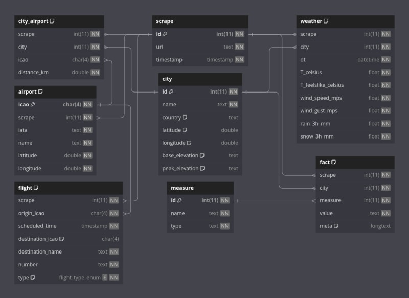
One of the results of this project is the SQL database schema which ended up like this and shows what data and what relations were acquired by the ETL:

Another result is the reports that were automatically generated, an example of which you can see here!

If you are reading this early enough, and I have not yet torn down the automation to save CPU, API and Google credits, you could see the actual page here!

And of course, finally, all the nice code and development notebooks:

• gans_cities_scraping_and_api.ipynb: notebook for developing the ETL and initial reporting
• gans_cities_scraping_and_api.py: refactored ETL code ready for use in the Google cloud-function
• main.py: the entry-point for the Google cloud-function driving ETL and reporting
• gans_update_report.py: code for making a new report from a Jupyter notebook template
• gans_cities_display.ipynb: Jupyter notebook used as the template for automatic reports

I did not do it

It would be cool to combine the flight data with the weather data. My idea would be to define sigmoidal functions that define the relative likelihood that people use E-scooters under different weather parameters, e.g. below a certain temperature, when it rains, snows or if the wind blows too strongly. With those, I could attenuate the usage predictions that I derived from the flight data or just use them individually to predict the flight-independent scooter activity. The missing piece here would be the "perfect weather curve" for usage over the day.

---

These were two packed weeks and even though, I have many years of software development experience, I learned a lot of new infrastructure and Python packages. I am also amazed at how my fellow boot campers are doing, most with a lot less prior experience!